Abstract
The role of multi-parametric (mp)MRI in the diagnosis and treatment of prostate cancer has increased considerably. An alternative to visual inspection of mpMRI is the evaluation using histogram-based (first order statistics) parameters and textural features (second order statistics). The aims of the present work were to investigate the relationship between benign and malignant sub-volumes of the prostate and textures obtained from mpMR images. The performance of tumor prediction was investigated based on the combination of histogram-based and textural parameters. Subsequently, the relative importance of mpMR images was assessed and the benefit of additional imaging analyzed. Finally, sub-structures based on the PI-RADS classification were investigated as potential regions to automatically detect maligned lesions. Twenty-five patients who received mpMRI prior to radical prostatectomy were included in the study. The imaging protocol included T2, DWI, and DCE. Delineation of tumor regions was performed based on pathological information. First and second order statistics were derived from each structure and for all image modalities. The resulting data were processed with multivariate analysis, using PCA (principal component analysis) and OPLS-DA (orthogonal partial least squares discriminant analysis) for separation of malignant and healthy tissue. PCA showed a clear difference between tumor and healthy regions in the peripheral zone for all investigated images. The predictive ability of the OPLS-DA models increased for all image modalities when first and second order statistics were combined. The predictive value reached a plateau after adding ADC and T2, and did not increase further with the addition of other image information. The present study indicates a distinct difference in the signatures between malign and benign prostate tissue. This is an absolute prerequisite for automatic tumor segmentation, but only the first step in that direction. For the specific identified signature, DCE did not add complementary information to T2 and ADC maps.
Export citation and abstract BibTeX RIS
Introduction
Multi-parametric magnetic resonance imaging (mpMRI) has become an important tool for diagnosis of prostate cancer over the last years, e.g. Kitajima et al (2010), Margolis (2014), Schoots et al (2015), Baur et al (2016), Polanec et al (2016a) and Thorwarth et al (2017). mpMRI includes T2-weighted (T2w) imaging, diffusion-weighted imaging (DWI), dynamic-contrast-enhanced MRI (DCE) and, as an optional technique, MR spectroscopy (e.g. PI-RADS II). All these imaging methods are meant to improve diagnostic accuracy by providing complementary information related to cell proliferation, hypoxia, perfusion or microvascular hyperpermeability (Georg et al 2015). According to a meta-analysis by de Rooij et al, the diagnostic accuracy of mpMRI for prostate cancer detection has a sensitivity of 74% and a specificity of 88% (de Rooij et al 2014). Thus, mpMRI could be an alternative to wide-scale prostate-specific antigen (PSA) screening, which leads to overdiagnosis and overtreatment (Alberts et al 2015).
With the increasing availability of MR scanners, mpMRI has started to influence radiation therapy (RT) as well (Dinh et al 2016). Studies have shown that the vast majority of the local recurrences after RT originate in the primary tumor (Cellini et al 2002, Pucar et al 2008). As the possibilities for further dose escalation to the whole prostate are limited due to toxicity in neighboring organs at risk (OARs) (i.e. rectum and bladder), an attractive option is to escalate the dose only to the volumes with higher tumor cell density. Improvements in the dose delivery to small targets and the possibility of combining irradiation techniques (e.g. external beam therapy with brachytherapy) make boosting imaging-defined dominant intraprostatic lesions (DILs) possible. Several strategies have been investigated where slight dose escalation to the DIL was performed (Bauman et al 2013, Sundahl et al 2016, von Eyben et al 2016). Currently at least two clinical trials are running in order to compare boost versus non-boost therapy in large patient cohorts (Lips et al 2011, Schild 2014).
The evaluation of mpMRI images of the prostate is mostly done by visual inspection, where lesions should be classified according to the established prostate imaging reporting and data system (PI-RADS) guidelines (Barentsz et al 2012, American College of Radiology 2015, Polanec et al 2016b). In some studies, an evaluation based on first order (gray level) statistics (i.e. histogram-based measures) was discussed, e.g. Lemasson et al (2013). First order gray level statistics represents the intensity distribution but lacks information about the spatial distribution and therefore also the full representation of the tumor heterogeneity. To overcome this limitation, second order statistics can be applied on mpMR images for diagnostic purposes (Chan et al 2003, Moradi et al 2012, Khalvati et al 2015, Kwak et al 2015, Wibmer et al 2015, Cameron et al 2016, Rampun et al 2016). Furthermore, textures were used for treatment response assessment studies e.g. for glioma patients (Brynolfsson et al 2014) and for tumor characterization studies, (e.g. Fox et al (2016)).
The large amount of information that is produced by using textural parameters requires multivariate analysis to handle the large number of variables. In PCA (principal component analysis), the high dimensionality of the data is reduced to a reasonable number of components. In most cases the projection into two or three principal components is sufficient. The underlying components can then be associated with one or several response variables in a second step. OPLS-DA (orthogonal partial least squares discriminant analysis) is a supplementary multivariate modeling technique, which fits a regression model between the multi-dimensional data and the response variables. OPLS-DA enables finding differences between two or more classes in an effective way. Subsequently, a model that discriminates observations from belonging to all but one class can be created (Trygg and Wold 2002). Both PCA and OPLS-DA can be said to belong to a typical chemometric workflow (Deming et al 1988), which aims to give the user a deeper understanding of the analyzed data through multivariate data analysis. This methodology is characterized by giving the user interpretable visualizations along with diagnostic tools for assessing the data e.g. Wu et al (2010). Although several of the regression tools used in the interdisciplinary field of chemometrics, e.g. OPLS-DA, could be classified as machine learning algorithms and hence are competing with techniques such as support vector machines and artificial neural networks, the aim of the chemometric methodology is not necessarily to achieve the highest performance. Instead, exploratory analysis with a high degree of interpretability is emphasized. Therefore, a chemometric procedure is often employed when the information content in the analyzed data is largely unknown.
Using textural features to analyze medical images is an upcoming research field, where many research questions remain to be solved (Coroller et al 2016, Brynolfsson et al 2017, van Timmeren et al 2017). The aims of the present work were to investigate the relationship between benign and malignant sub-volumes of the prostate and textures obtained from mpMR images, including its assessment and quantification. More specifically, the combination of histogram-based and textural parameters with respect to their performance in tumor prediction was investigated with statistical methods and the relative importance of mpMR images was assessed. In this context, the benefit of additional mpMR imaging was analyzed because today's imaging protocols tend to include as many sequences as possible, which in turn affects workload. Finally, sub-structures based on the well-established PI-RADS classification were investigated as potential regions to automatically find maligned lesions in the peripheral zone of the prostate.
Material and methods
Dataset
In total, 25 patients from a multimodal imaging study, which was approved by the local institutional review board, were included in the presented study. The inclusion criterion for this sub study was radical prostatectomy which was decided on in mutual agreement between physician and patient. Exclusion criteria for the multimodal imaging study in general were contraindication for MRI or contrast agents. The median patient age was 63 years (ranging from 46 to 74 years). All patients were prescribed with an mpMRI based on one or more of the following criteria: elevated prostate-specific antigen (PSA) levels >4.0 ng ml−1; suspicious findings upon digital rectal examination or transrectal ultrasound (TRUS); and/or biopsy-based histopathological evaluation. All surgeries were conducted between March 2012 and August 2014.
The patients did not receive hormonal or any other prostate therapy (or therapy to other organs in close proximity) prior to the mpMRI. In the histopathological evaluation, 11 patients were rated with a Gleason score (GS) of 6 (3 + 3), 14 patients had a GS of 7 (4 + 3) and one a GS of 9 (5 + 4). The mean PSA level was 9.0 ng ml−1 (ranging from 1.7 to 39.2 ng ml−1). In the investigated patient cohort, 10 patients had one dominant intraprostatic lesion (DIL) in the peripheral zone (PZ), 13 patients 2 DILs, and 2 patients had 3 or more DILs in the PZ. Nine patients had one or more lesions in the central gland (CG).
The mpMRI was performed on a 3T MAGNETOM TimTrio MRI (Siemens Healthcare, Erlangen, Germany), with combined spine and body array receive coils (no endorectal coil). The patients were asked to empty their bladders before the imaging procedure and then an intestinal lavage was performed. The patients' rectums were thereafter filled with ultrasound gel (Gello GmbH, Germany). All patients were administered with 10 mg of Hyoscine butyl-bromide (Buscopan, Boehringer Ingelheim, GmbH, Germany) to suppress peristalsis motion. In order to perform contrast enhanced imaging, Gadoteratemeglumine (Gd-DOTA, Dotarem, Guerbet, France) was injected intravenously as a bolus of 0.2 ml per kg of body weight using a power injector at 4 ml s−1 followed by a 20 ml saline flush after three baseline scans. All scans were conducted in a feet first supine position.
The imaging protocol consisted of the following sequences (see also table 1):
- anatomical high resolution T2-weighted turbo spin echo (TSE) in all three planes (hereafter denoted as T2w);
- diffusion-weighted, single-shot echo-planar imaging (DWI) with inversion recovery fat suppression, for which the apparent diffusion coefficient (ADC) maps were calculated directly in the scanner software. DWI was performed with four b-values and all were used for generation of the ADC map: 0, 100, 400, and 800 s mm−1;
- dynamic contrast enhanced (DCE)-MRI, using a view-sharing 3D T1-weighted gradient echo sequence (TWIST);
- k-space subsampling with central region 30% and sampling density 25% resulting in a temporal resolution of 4.22 s;
Table 1. Overview of the settings used for mpMRI. TR and TE are the repetition time and echo time, respectively. FOV is the field of view; the slice thickness was 3.6 mm for all sequences. The last column gives sequence-specific information. For DWI b values were 100/400/800 s mm–1.
| Protocol | TR (ms) | TE (ms) | FOV (mm) | Flip angle (deg) | Grappa factor | Averages | Matrix | |
|---|---|---|---|---|---|---|---|---|
| T2w TSE | 4000 | 101 | 200 × 200 | 150 | 2 | 3 | 320 | |
| DWI | 3300 | 60 | 260 × 260 | 90 | 2 | 8 | 160 | SPAIR fat suppression |
| T1w gradient echo twist | 3.85 | 1.42 | 260 × 260 | 12 | 2 | 1 | 160 | DCE with 70 repetitions |
The Syngo Tissue 4D image post processing platform (Siemens) was used to generate the Ktrans and iAUC maps. For Ktrans modeling the Tofts model with non-linear fitting was utilized. A pixel wise calculation for Ktrans was applied without smoothing in post processing. The DCE MRI series were aligned prior to modeling to correct for prostate movements (internal Tissue 4D correction algorithm was used and the results were visually checked by the physician). The contrast agent specific parameters like molarity and relativity were automatically determined by the used contrast agent (software adjusts these values based on chosen contrast agent). The volume of injected contrast was set accordingly for each patient, based on the patient's weight. The arterial input function (AIF) was set to fast. The contrast agent arrival time was detected automatically and visually inspected. No T1 mapping was applied, and a fixed T1 value (1500 ms) was used.
Also in this study, three time points of the above described T1w-DCE modality were further investigated: before the contrast agent was administered (henceforth labeled T1w), 79 s after administration (i.e. the average peak time point and hereafter labeled DCEEarly), and at t = 300 s (i.e DCELate).
The correction for motion during a dynamic sequence was performed using Syngo Tissue 4D tool and the alignment between all image modalities and imaging derived parameters was performed offline using the imaging software MIRADA RTx (Mirada Medical, Oxford, UK) applying automatic rigid registration followed by manual corrections. Furthermore, all images were corrected for gradient non-linearities using scanner's vendor package.
In addition all images were rigidly registered to the T2w MRI (automatic tool followed by manual corrections) and resampled to the voxel size of the T2w image (i.e 0.625 × 0.625 × 3.60 mm3) using the imaging software Mirada RTx (Mirada Medical, Oxford, UK). The dynamic scans were corrected for motion using rigid registration.
The radical prostatectomy specimens were cut perpendicular to the Denonvilliers' fascia from the base to the apex with a thickness of 4 mm using a cutting device. After embedding the slices in paraffin, the whole mount sections were stained with H&E. Areas of prostate cancer were tagged by a pathologist under the microscope. The sets of slices were scanned using a document scanner with high resolution in a 1:1 scale (see figure 1).

Figure 1. (a) Delineation on T2w MRI; (b) geometrical substructures in the CG and PZ; (c) slice of resected prostate with marked tumor region.
Download figure:
Standard image High-resolution imageDelineation
Delineation of the anatomical structures (i.e. CG and PZ) was performed by two radiation oncologists (with 12 and 3 years of experience in prostate radiotherapy) on the T2w images using the Mirada RTx software. Furthermore, the tumor regions were delineated based on the pathological information by visual comparison by the radiation oncologists. Delineated structures were subsequently transferred to all image modalities and imaging derived parameter maps; 'tumor-only' regions were compared with 'healthy tissue' regions. As visual comparison between MRI and the pathological images is challenging (Meyer et al 2013, Kalavagunta et al 2015, McGrath et al 2016), regions of uncertain diagnostic assignment around the tumor were excluded from further processing. For patients with large tumor volumes, the normal tissue was sometimes separated into two or more sub-regions due to software limitations. These regions were subsequently analyzed separately. Thus, in total 92 structures were processed for each image modality.
In addition to the 'tumor-only' and 'healthy tissue' structures, the CG and PZ were divided into geometrical substructures. These substructures were based on those used in the PIRADS classification (American College of Radiology 2015) and are depicted in figure 1. In total 22 of these substructures were delineated for each patient (6 in CG and 16 in PZ). Based on the pathological information, these geometrical substructures were scored in four distinct levels, i.e. T/H1 (lowest score), T/H2, T/H3, and T/H4 (highest score), by the radiation oncologists. The scores were given in accordance to the tumor prominence and area of the region occupied by tumor tissue, in agreement with the PI-RADS scoring guidelines (American College of Radiology 2015). The aim of this approach was to test models for tumor prediction.
The presented study investigated only tumors in the PZ as only 20% of all tumors occurred in the CG. This is a typical ratio of prostate cancer occurrences between CG and PZ (McNeal et al 1988, Vargas et al 2012).
Data analysis
Textural information of the ROIs described above was generated using gray-level co-occurrence matrices (GLCMs) (Haralick et al 1973, Yang et al 2012). The GLCMs were computed with bin sizes of 8, 16, and 32 in four directions (i.e. vertical, horizontal and two diagonals) with the combined information of all four directions was being used subsequently. The range of gray level binning was based on values between the 2% gray value level and the 98% gray value level of each patient.
GLCMs were calculated separately for each slice and summed up before further processing. Based on the GLCMs, 9 textural measures (i.e. second order statistics) were calculated and further processed for each image modality in transversal planes.
Data processing was performed using MatLab (R2013a, 64 bit MathWorks, Natick, Massachusetts USA). For the GLCMs, the following textural features were calculated using the Image Processing Toolbox extension by Brynolfsson (2016): autocorrelation, cluster prominence, cluster shade, energy, maximum probability, sum average, sum entropy, sum of squares variances, and sum variance. The mathematical expressions of these features are listed in table 2 of the appendix and are described in detail in the work by Haralick et al (1973) and Soh and Tsatsoulis (1999). Thus, the term 'Haralick features' is also used in the following. The remaining 10 Haralick features were not used, as they correlated with the volumes of the investigated structures, as outlined in the discussion.
Table 2. Mathematical expression of the applied textural features.
| Feature | Equation |
|---|---|
| Energy |  |
| Auto correlation |  |
| Cluster prominence |  |
| Cluster shade |  |
| Maximum probability |  |
| Sum of squares variance |  |
| Sum average |  |
| Sum variance |  |
| Sum entropy |  |
Furthermore, based on the gray value histogram of each image modality, the following nine parameters (first order statistics) were processed for each volume of interest (VOI) and normalized to the mean gray value of each PZ: mean, median, standard deviation, skewness, kurtosis, 2nd percentile, 15th percentile, 85th percentile, and 98th percentile (Just 2014).
For all image modalities and imaging derived parameter maps, the Haralick features were assembled in separate matrices Xi. The size of Xi was 94 × 27, where 94 is the number of observations (i.e. tumor and healthy structures). Note that each of the nine Haralick features was calculated for three different GLCM bin sizes. Furthermore, seven matrices were assembled for the nine first order statistic parameters (Xj), with a size of 94 × 9.
Unsupervised modeling of first and second order statistics
The multidimensional data, i.e. matrices Xi and Xj, were analyzed with PCA (Wold et al 1987) using the software SIMCA (SIMCA 14, MKS Umetrics, Umeå, Sweden). PCA compresses a multidimensional data set with correlated variables into fewer orthogonal and uncorrelated variables, so-called principal components. PCA represents an unsupervised data modeling methodology without the influence of a response variable, details can be found in the appendix.
As PCA obtains a set of score vectors from the original variables, these can be used as input in scatter plots, which reveal the majority of variation in the analyzed data. The score plot is usually created for the first two score vectors t1 and t2. It shows the variation in the data compressed into a 2D plane. PCA score plots can give information about outliers, non-linear relationships in the data, and most importantly, how similar the observations are to each other. It can therefore be beneficial to explore a previously non-analyzed data set with PCA prior to further modeling with various machine learning methods, such as support vector machines or artificial neural networks, which typically use an external response variable for classification or regression (Jain et al 2000).
For all image modalities available in this study, score scatter plots of the first and second order statistics were assessed visually for differences between tumor and healthy tissue. The number of plotted points equaled the number of observations and corresponded to the number of processed structures, i.e. 94. Scatter plots from models based on the predefined geometrical substructures, which typically showed a subtle difference between structures with and without tumor presence, were further analyzed with receiver operating characteristic (ROC) curves in order to describe the strength of the observed relationship. The basis for the ROC analysis was the first two components of each PCA model created for the different image modalities. A direction in the score space that spanned the difference between tumor and healthy structures was then set. The position for each of the observations along this regression line was used as an input for the ROC analysis. Thus, a certain point at the line will correspond to a certain sensitivity and specificity. As a consequence, the regression in score space equaled principal component regression (PCR) (Frank and Friedman 1993). Finally, for each of the models, the area under the curve was derived as a measure of the difference between tumor and healthy structures.
Supervised modeling of first and second order statistics
In addition to the unsupervised PCA modeling, a specific multivariate regression technique, i.e. orthogonal partial least squares discriminant analysis (OPLS-DA), was used to assess the relationship between the X matrices and a response y, representing the pathological information of the prostate structures (Trygg and Wold 2002, Bylesjö et al 2006). Thus, the OPLS-DA decomposition can be seen as:


 and
and  are the transposed mean vectors of X and y. X is decomposed into the y-correlated single component tp' and the orthogonal components T0P0. E and f depict the variation that cannot be explained by the model, i.e. the residual. OPLS-DA removes variation in X that is orthogonal to the response (i.e. T0P0) by subtracting these components from X. It then fits a model between X and y. The response y is then obtained with the correlated transposed component tq', where q is the loading vector of the response y. The length of the vector y is 94, which is the number of observations. For the OPLS-DA modeling, the response y was set to one for tumor structures and zero for healthy structures.
The quality of an OPLS-DA model was assessed quantitatively by R2Y and Q2Y (Eriksson et al 2013). Mathematically R²Y and Q²Y are outlined in detail in the appendix.
OPLS-DA is only presented for stronger relationships between the matrices X (first and second order statistics) and the response y (tumor presence), specifically, if Q²Y exceeded a value of 0.2. For the evaluation of the geometrical substructures, which are based on the PI-RADS classification, Q²Y values close to zero were obtained. Thus, only the OPLS-DA results of tumor-only versus healthy tissue were reported in the results section.
Workflow of data analysis
As illustrated in figure 2 in the left flowchart, tumor-only and healthy structures were processed as described above. The multidimensional data (i.e. Xi and Xj) were the input for the described models (i.e. PCA and OPLS-DA). Using the predictive ability (Q²Y) of the OPLS-DA first and second order statistics was compared as model input, separately for all seven image modalities. Furthermore, the benefit of using first and second order statistics in combination was evaluated. The quantitative parameter Q²Y was also used to evaluate the additional benefit of multi-parametric imaging of the prostate for tumor diagnostics. Therefore, the T2w image modality was chosen as a starting point, as this sequence is currently standard in MR imaging and will remain as such in the imaging workflow.

Figure 2. Illustration of the steps of the study. The left side indicates the process of evaluating tumor-only and healthy structures, while on the right side, the process of geometrical substructure evaluation is shown.
Download figure:
Standard image High-resolution imageThe geometrical substructures, including their score (i.e. T/H1 to T/H4), were processed in the same way as tumor-only and healthy structures (see figure 2), with the aim to use these well-established structure designs to predict tumor presence. As outlined in the discussion section, this prediction was challenging, and thus OPLS-DA results are not reported. Instead, the area under the ROC curves is given for the structures with different tumor scores.
Results
The results section is organized as follows: separation models for tumor and healthy structures by means of principal component analysis (PCA) and orthogonal partial least squares discriminant analysis (OPLS-DA) are presented in the first section, while the second part includes data on the predefined geometrical substructures and the potential prediction of tumor occurrences in these structures.
Separation models for tumor and healthy structures
Non-supervised PCA was applied on the first and second order statistics to generate score scatter plots where the differences between tumor and tumor-free regions could be assessed. The strongest relationship was observed for the model based on ADC data (see figure 3). Here tumor observations were largely separated from healthy tissue in the first component t1 which explained 43.1% of the variance in the data. The second component t2 (explaining 20.7% of the variation) appeared to predominantly host intra-group variation and did not contribute to the separation between the groups. Similar scatter plots, regarding visual separation, were obtained for T2w images followed by Ktrans and iAUC. Weaker relationships, characterized by a more overlapping appearance of the two groups, were found for T1w, DCEEarly, and DCELate. Some moderate outliers, which were still kept in the models, resided outside the Hotelling ellipse in some of the modalities, for example ADC (see figure 3).

Figure 3. Left: scatter plot for ADC map model showing the difference between tumor regions (red circles) and healthy tissue (blue crosses). The PCA is based on parameters derived from first and second order statistics. The ellipse in the scatter plot represents the Hotelling's T2 statistics. Right: 1D projection of the score scatter plot, only showing the first principal component.
Download figure:
Standard image High-resolution imageThe distinct difference between tumor and healthy tissue, as seen in the PCA modeling, was explored with OPLS-DA. The results of these models are exemplified through a scatter plot for ADC values, as shown in figure 4, including both first and second order statistics. This figure illustrates the appearance of the predicted tumor and healthy tissue observations in the model score space since there is almost a clear separation between the two classes.
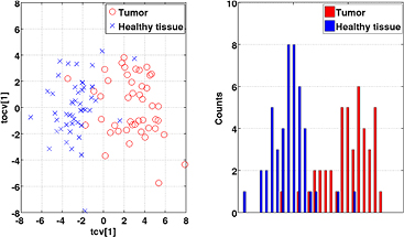
Figure 4. Left: score plot for the OPLS-DA model of tumor (red circles) versus healthy structures (blue crosses) for the ADC modality using first and second order statistics. The cross-validated score values of the predictive component, tcv[1], can be seen on the x-axis. The second component corresponds to the first orthogonal component, tocv[1]. Right: 1D illustration of the OPLS-DA model projected to the predictive component tcv[1].
Download figure:
Standard image High-resolution imageTo evaluate the OPLS-DA model for the different image modalities and derived parameters, R2Y and Q²Y values were calculated (see equations (A.5)–(A.7)). For each image modality and imaging derived parameter map, three models were created based on (1) first order statistics; (2) second order statistics, and (3) the combination of both. The predictive ability (Q²Y) of each model is shown in figure 5. The use of second order statistics did improve the predictive ability by 23% compared to using first order statistics only. The combination of both statistics improved the predictive ability by 54% compared to using first or second order statistics separately. Both values are the average value of all seven image modalities. For individual image modalities, the combination of both statistics improved the Q²Y value in all cases compared to using first or second order statistics only. The improvement ranged from 5% up to a factor of 3.2. Detailed values for Q²Y and R²Y are given in the appendix (figure 9).
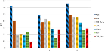
Figure 5. Predictive ability (Q²Y) obtained with OPLS-DA in comparison for first (I) and, second order statistics (II), and in combination (I + II), for different image modalities and parameter maps.
Download figure:
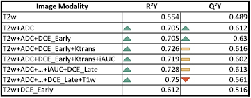
Standard image High-resolution imageIn figure 6, the model fit, R2Y, and the predictive ability, Q²Y, of the OPLS-DA model are given for a range of increased complexity as far as the included images are concerned. The Q²Y value increased by 25% by adding ADC map to T2w as model input. Adding DCEEarly only increased the predictive ability by another 3%. The addition of Ktrans and iAUC to the model lowered the predictive ability. The exact values are given in the appendix (figure 10).
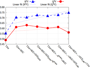
Figure 6. Model fit (R²Y) and predictive ability (Q²Y) for various combinations of images. The additional information gained by multiple imaging reached a plateau after adding ADC map to T2w (red line).
Download figure:
Standard image High-resolution imageEvaluation of geometrical substructures in the peripheral zone of the prostate
PCA models were created for geometrical substructures of the PZ (peripheral zone) based on the various image modalities and imaging derived parameter maps. As an example, the scatter plot for the ADC map is shown in figure 7. Overall, these scatter plots revealed only weak relationships between geometrical substructures of different tumor scores. These relationships corresponded to a visual appearance with completely overlapping tumor scores. Only for the highest tumor score (i.e. T/H4, represented as squares in figure 7) the observations were predominantly located on the left side of the scatter plot.
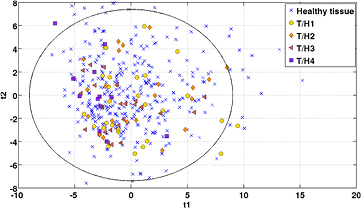
Figure 7. Score scatter plot of the first and second components (explaining 37.5% and 25.1% of the variance) for the ADC map model illustrating the predefined geometrical substructures. Blue crosses symbolize the structures without any tumor occurrence while the other symbols reflect a certain tumor score, where T/H1 represents the lowest score and T/H4 the highest. The PCA is based on parameters derived from first and second order statistics. The ellipse in the scatter plot represents the Hotelling's T2 statistics.
Download figure:
Standard image High-resolution imageROC curves were calculated for T2w, ADC, and DCEEarly. The area under the curve values for the ROC analysis are summarized in figure 8. For delineated substructures with the two smallest tumor proportions (i.e. T/H1 and T/H2), the values of the area under the curve are close to 0.5, with the only exceptions being the second order statistics and the combined statistics of T2w. For the highest tumor to healthy tissue ratio (i.e. T/H 4), the area under the curve reaches values of up to 0.83 (for ADC). A clear difference between the usage of first order, second order or combined statistics could not be observed.
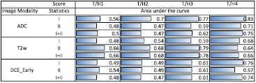
Figure 8. ROC curves obtained by the unsupervised PCA modeling for ADC map, T2w, and DCEEarly the area under the curve was first calculated separately for first and second order statistics (labeled as 'I' and 'II'), as well as for the combination of both ('I + II') for all four tumor scores (T/H1 − T/H4).
Download figure:
Standard image High-resolution imageDiscussion
Scientific interest is growing in using textural features for the evaluation of medical images, e.g. Lambin et al (2012), Kumar et al (2012) and Parmar et al (2014), but it is still far from being a standardized technique to process mpMRIs. There are only a few publications addressing texture analysis for prostate cancer (Chan et al 2003, Moradi et al 2012, Khalvati et al 2015, Kwak et al 2015, Wibmer et al 2015, Rampun et al 2016). The details on how textural features were utilized and which features were employed vary between the different studies. Furthermore, many publications investigate only one mpMRI sequence. In the presented study all major MRI modalities and imaging derived parameter maps for prostate cancer were considered, with the exception of MR spectroscopy, which is seen as an optional parameter (Polanec et al 2016a).
Gray-level co-occurance matrices (GLCMs) are needed as input to calculate the parameters of the second order statistics. These matrices can be calculated in different ways. For example, orientation and bin size can be varied, resulting in different GLCMs and thus in different values for the textural features. The presented results in this study were based on GLCMs calculated using three different bin sizes (i.e. 8, 16, and 32). However, models based only on one of the previously mentioned bin sizes resulted in very similar prediction values. Using four orientations (i.e. vertical, horizontal and two diagonals) in the GLCM calculation produced denser matrices and thus a more robust generation of the derived Haralick textural features.
The textural parameters derived using the Matlab toolbox were based on the work by Haralick et al (1973) and Soh and Tsatsoulis (1999). Thus, not only the 9 textural parameters mentioned above were calculated, but 19 in total. However, eleven of those textural features showed a potential dependency on the size of the processed structure. As the size of the processed structures varied from small malignant lesions to structures nearly as big as the peripheral zone (PZ) itself, such parameters had to be excluded from further processing as they would have a high impact on the models. A detailed investigation of this issue was not within the scope of this study. To the authors' knowledge, such dependency is not described thoroughly in the literature for MRI, but is reported for the evaluation of PET images of a NEMA phantom (Nyflot et al 2015). In general, textures can also be affected by imaging parameters such as noise or resolution (Brynolfsson et al 2017). In this study the Haralick features were calculated based on summed up 2D GLCMs. Brynolfsson et al showed that the difference in the textural features of different planes is minor as well as the sensitivity to voxel size variation. Using 3D textural analysis instead of 2D could result in an improved model, as for example shown by Fetit et al for conventional MR images in childhood brain tumors, where the overall accuracy of a neural network classifier improved by 19% (Fetit et al 2015). However, if this is also valid for the presented models remains to be investigated in detail. In our study, small tumor sizes of down to two slices are challenging this approach due to sparse GLCMs.
The advantage of the multivariate methods used in this paper is the possibility to process large numbers of variables present in the X matrices as both techniques are suitable for modeling variables with high collinearity (Bharati et al 2004). However, in cases where serious collinearity problems exit, for example when the number of predictor variables by far exceeds the number of observations, it can be advantageous to use shrinkage operators (e.g. LASSO) to effectively reduce the number of variables (Acharjee 2012, Pavlou et al 2016). This was not the case, however, in our study for orthogonal partial least squares discriminant analysis (OPLS-DA) and prinicipal component analysis (PCA), as the number of variables was comparatively low, far too low to test the limits of OPLS-DA.
As all PCA score plots demonstrating a linear relationship between the presence of tumor and the plotted score values, with a trend going in a single direction, OPLS-DA was deemed to be a good candidate for handling the regression modeling between tumor-only and tumor-free structures. As PLS and its siblings, OPLS and OPLS-DA, normally fit linear models between the predictor variables X and the response y, there may be instances where other machine learning techniques are better suited. This could especially be the case when non-linear relationships are observed. In the future, other machine learning techniques could be tried on the data presented in the current study. However, the aim of the study was to investigate the relationships in an exploratory manner and to provide give an initial assessment.
Using the predictive ability of the OPLS-DA modeling as a measure showed that for some image modalities and imaging derived parameter maps, models based on first order statistics are superior to models based on second order statistics (ADC, T1w), while for others models based on second order statistics are in favor (Ktrans, DCEEarly, DCELate, iAUC) (see figures 5 and 9). Both models for T2w resulted in similar predictive values. For all investigated images, the combination of first and second order statistics improved the prediction value of the models (i.e. Q²Y). Ranging from 5% compared to ADC first order statistics to 220% compared with DCELate first order statistics (see figures 5 and 9). This indicates that first and second order statistics provide complementary information and should both be included in a multivariate prediction model to maximize the predictive ability.
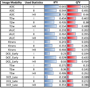
Figure 9. Predictive abilty (Q²Y) and goodness of the OPLS model (R²Y) for all investigated image modalities and parameter maps. For each image type both values were calculated based on first order statistics (I), second order statistics (II), as well as the combination of first and second order statistics (I + II).
Download figure:
Standard image High-resolution imageIt has to be highlighted that the quality of DCE MRI could be improved by more sophisticated settings during the scans. In this study, established general clinical parameters were used, as described in the section material and methods. Regarding the influence of different methods of constructing ADC maps on textural measures, a recent study by Brynolfsson et al showed that this has no impact on any textural features (Brynolfsson et al 2017). The registration between pathological information and MRI can be another source of uncertainty of unknown magnitude. As outlined above several studies report on registration difficulties between pathological slices and MRI due to differences in in- and ex vivo conditions of the prostate.
By using OPLS-DA, it was also possible to investigate the additional benefits of multiparametric imaging. The Q²Y parameter gives the predictive ability, in contrast to the R²Y value which gives the goodness of fit. R²Y increases by adding more parameters to the model, while Q²Y only increases if the information is complementary (see figure 6). According to the presented OPLS-DA model, the additional benefit for adding DCE, Ktrans, and iAUC to the model is very limited (<3% increase of predictive ability) (see figures 6 and 10). In figure 6 it can be observed, that the predictive power Q²Y even decreases from 0.60 to 0.55 when adding the T1w image modality, which is caused by non-predictive variation (see equations (A.5)–(A.8)). Note that especially DCE modeling is a complex process and its results may vary depending on the used settings. The fact that the imaging protocols for prostate cancer are so manifold nowadays means the workload for the clinical personnel as well as for the patients increases. This highlights the need for continuous evaluation of which sequences to include in the clinical imaging protocols. For the specific aim of detecting an intra-prostatic lesion in the peripheral zone the present study indicates that DCE seems to provide less information compared to ADC maps when added to T2w. This is supported by the fact, that the predictive power (Q²Y) of T2w plus DCEEarly was only 0.512, which is 0.096 less than T2 plus ADC (see figure 10). However, it has to be pointed out that 25 patients are not enough to consider these as definite findings.
Figure 10. Predictive ability (Q²Y) and goodness of the OPLS model (R²Y) when combining image types. Green arrows symbolize an increase in comparison to the value of the row above, while red arrows represent the opposite. Yellow bars indicate a change of less than 3% compared to the value in the line above. Additionally, the combination of T2w and DCEEarly was calculated.
Download figure:
Standard image High-resolution image
In a multivariate OnPLS analysis, an extension of OPLS that works for several data blocks (Löfstedt et al 2013), the T2w images, ADC, and DCEEarly showed that only the redundant model components of contained variances were related to the prediction of tumor and healthy tissue.
As indicated above, the benefit of OPLS-DA was proven for stronger relationships between the derived features in matrix X and the response y. The quantitative measure Q2Y which normally obtains a value between 0 and 1, was consequently reported for stronger relationships with values above 0.2. A value close to 0 means no predictive ability, which corresponds to a visual appearance of the score plot where the two examined classes are completely overlapping and show a large intra-class spread. On the other hand, a Q2Y value of close to 1 means perfect predictive ability where the visual appearance of the corresponding score plot would be two completely separated classes with almost no intra class spread. Consequently, Q2Y is a comprehensive measure as it considers the overall spread of the predicted class. The highest Q2Y values reported in this study were above 0.6, and can be considered to represent strong relationships with mostly separated classes and controlled intra class spreads. This can also be seen in the score plots, exemplified by figure 4.
The number of correct observations can be extracted from the cross-validation and represents an alternative quantifying measure. However, these values are not reported in the present study as our aim was not to build a model for classification. For the sake of comparison, the best models obtained a classification rate of 85 out of 92 (92.4%). Furthermore, using the described ROC analysis on the cross-validated OPLS-DA score values, the predictive ability of the best models can be translated into area under curve values between 0.96 and 0.97, which is close to the perfect model (i.e. area under the curve of 1) (Fawcett 2006).
For the predefined geometrical substructures, based on the PI-RADS classification, the obtained Q²Y values were close to zero or in some instances negative. The latter indicates a poorer classification rate than that given by pure chance. As illustrated in figure 7, the observations belonging to the different tumor to healthy tissue ratio classes were overlapping. For these, ROC analysis on a simple regression in the PCA score space of the first two components was used to assess the relationships. The obtained area under the curve values also showed poor results (i.e. close to a classification rate of pure chance). These findings indicate that the pre-defined substructures, are not suitable to classify the regions with respect to their tumor presence. As decisions in radiology are often based on the PI-RADS classification system, the failure of using the underling substructures of tumor prediction models can still be considered an essential finding.
The present study indicates a distinct difference between the signatures (first and second order statistics) of malign and benign prostate tissue. The delineated tumor-only regions, which were pathologically confirmed, were clearly separated from the healthy regions in the PZ of the prostate with the presented models. This is an absolute pre-requisite for automatic segmentation, but only the first step in that direction. The statistical methods combined with first and second order statistics used in the present work were not able to separate healthy tissue from geometrical sub volumes with a smaller amount of tumor involvement (see figure 7). As we were able to clearly differentiate between tumor and healthy tissue, it appears that the failure with geometrical sub volume classification is mainly due to a lack of sensitivity of the features over larger mixed volumes. Moving towards local textural features could potentially address this issue.
Conclusion
This study shows that both first and second order statistics extracted from mpMRI data could be used to differentiate between tumor and healthy tissue in the peripheral zone of the prostate. T2w and ADC turned out to be the important image information for the OPLS-DA model used, while DCE did not contribute essential complementary information. This finding should be investigated in more detail with respect to mpMR imaging protocols. Furthermore, the combination of histogram-based and textural parameters increased the prediction availability in the presented models for all imaging modalities. An attempt to classify larger geometrical substructures, as utilized in the PI-RADS classification, with respect to the presence of tumor tissue failed, which indicates that the image features may need to be calculated more locally.
Acknowledgments
The financial support by the Austrian Federal Ministry of Science, Research and Economy and the National Foundation for Research, Technology and Development is gratefully acknowledged. The authors would like to thank Dr Georg Lösch for providing some of the pathological slices.
Conflict of interest
The authors have no relevant conflicts of interest to disclose.
Appendix
The purpose of this appendix is to provide more details on the mathematical background on PCA and OPLS-DA. Furthermore, information regarding the mathematical expression of the applied textural features are provided as well as two tables providing detailed information on the Q²Y and R²Y values for each investigated model.
Appendix. Unsupervised modeling
Mathematically, the unsupervised modeling for the decomposition of matrix X into its principal components is given in equation (A.1). T is the matrix of score vectors (ti), and P the matrix of loading vectors (pi), with E being the residual. The apostrophe indicates a transposed matrix.

Further, TPʹ can be written as the sum over N score vectors and loading vectors, respectively, where N is the number of observations.

Geometrically, each loading vector p can be defined as the projection of the columns of matrix X onto a score vector t as follows

By projecting the rows of matrix X onto the loading vector p, the score vector is given as

In the NIPALS algorithm (Wold 1966) for calculating PCA, an arbitrary column vector of X is selected as the initial score vector t. Then the vectors t and p are derived iteratively until they reach the threshold (i.e. 10−7). After a component has been calculated, it is subtracted from X and a new component is calculated from the residual. The size of each computed score vector t corresponds to the number of observations (i.e. 94, the number of structures), and the size of the loading vector p corresponds to the number of variables, which is 9 for the first order statistics and 27 for the second order statistics evaluation.
Appendix. Supervised modeling
R2Y is a measure of how well the response y can be fitted by the predictor variables in X (i.e. the first and second order statistics). It can be calculated as

where SST is the total sum of squares (variance) in the data and SSR is the residual sum of squares. Thus, SSR is calculated on the residuals after the model has been fitted from the observed (yi) and model calculated response values (ycalc,i) for all observations N (N = 94) as

The mathematical expression for Q2Y is similar to that of R2Y, but is calculated as a quantitative measure of model predictive ability as

PRESS is calculated as the prediction error sum of squares from the observed response values  and the predicted response values
  as
as

PRESS and Q2Y are obtained from cross-validation where a certain number of observations are omitted from modeling and are then predicted by the model. In the current work, we have employed a cross-validation procedure in which all structures from the same patient were left out at the same time to ensure no redundancy remains in the data when performing the prediction. Both quality parameters (i.e. R2Y and Q2Y) range from 0 to 1, where a value of 1 implies perfect model fit, i.e. perfect prediction, whereas a value of 0 means a completely unfitted model or no predictive ability (Eriksson et al 2013).
Appendix. Textural features
The mathematical expressions given in table 2 use the notations given in equations (A.9)–(A.12), where p(i, j) is the (i, j) entry of the GLCM and Ng is the number of gray levels.


µ in equations (A.9) and (A.10) is the mean of the rows (µx) and columns (µy) of the GLCM. Further, for symmetric GLCMs

As defined in Haralick et al (1973) the variable px+y(k) sums probabilities diagonally, where  .
.