

Abstract
The severity and timing of seasonal malaria epidemics is strongly linked with temperature and rainfall. Advance warning of meteorological conditions from seasonal climate models can therefore potentially anticipate unusually strong epidemic events, building resilience and adapting to possible changes in the frequency of such events. Here we present validation of a process-based, dynamic malaria model driven by hindcasts from a state-of-the-art seasonal climate model from the European Centre for Medium-Range Weather Forecasts. We validate the climate and malaria models against observed meteorological and incidence data for Botswana over the period 1982–2006; the longest record of observed incidence data which has been used to validate a modeling system of this kind. We consider the impact of climate model biases, the relationship between climate and epidemiological predictability and the potential for skillful malaria forecasts. Forecast skill is demonstrated for upper tercile malaria incidence for the Botswana malaria season (January–May), using forecasts issued at the start of November; the forecast system anticipates six out of the seven upper tercile malaria seasons in the observational period. The length of the validation time series gives confidence in the conclusion that it is possible to make reliable forecasts of seasonal malaria risk, forming a key part of a health early warning system for Botswana and contributing to efforts to adapt to climate change.
Export citation and abstract BibTeX RIS

Content from this work may be used under the terms of the Creative Commons Attribution 3.0 licence. Any further distribution of this work must maintain attribution to the author(s) and the title of the work, journal citation and DOI.
1. Introduction
Malaria is a mosquito-borne infectious disease caused by parasitic protozoans of the Plasmodium genus. It has a detrimental socio-economic impact on affected countries, presenting a significant public health challenge, and it is inextricably linked with poverty. Approximately half of the world's population is at risk of malaria, with approximately 198 million reported cases and an estimated 584 000 reported deaths in 2013 (World Health Organization 2014). Most deaths occur among children living in Africa, where a child dies every minute from malaria, with the majority of cases in epidemic areas, where the human population has little or no immunity to the parasite (Worrall et al 2004).
Malaria is ranked as a major public health problem in Botswana despite a national malaria control program dating back to the 1970s (Thomson et al 2006). Since the 1980s malaria epidemics in the countries of Southern Africa have become more frequent and severe due to a combination of factors including environmental changes, drug resistance, population movements and social issues affecting the efficacy of control measures (Mabaso et al 2004). In Botswana, climate variability has been found to be a strong driver of malaria incidence variability; studies have shown that variability in December–January–February average (DJF) rainfall totals accounts for more than two-thirds of the inter-annual variability in standardized malaria incidence (Thomson et al 2005).
Climate variables such as temperature and rainfall are closely linked to the cycle of malaria development and infection and influence the life cycles of the Plasmodium parasite and the female Anopheles mosquito vector. The climatic conditions also influence vector breeding site availability (through enhanced rainfall) and the rate of disease transmission (through increased frequency of mosquito biting) (Morse et al 2005, Jones and Morse 2010, 2012). Epidemic outbreaks can occur as a result of climate anomalies, such as prolonged periods of rainfall or heat waves, particularly in regions where malaria transmission is strongly seasonal (Najera et al 1998, Worrall et al 2004, Protopopoff et al 2009). However the relationship between meteorological variables and malaria is nonlinear: although water is necessary to form mosquito breeding sites, excess rainfall and flooding can lead to flushing of larvae (Paaijmans et al 2007). Similarly increased temperature increases the rate of parasite and vector replication, but extreme temperatures reduces their respective survival rates and the overall vectorial capacity (Paaijmans et al 2012)
Climate models run in seasonal forecasting mode can potentially provide information regarding upcoming seasonal climate anomalies. These models simulate the dynamical evolution of atmospheric and oceanic initial states in the same way as is done in weather forecasting, but with a much longer timescale; generally they forecast conditions several months ahead. Predictability on these timescales comes from low-frequency aspects of the climate system, such as the ocean or the land surface (Troccoli 2010). By employing dynamic disease models simulating all stages of the transmission process based on weather conditions and driving such models with seasonal climate forecasts, there is potential to predict the risk of malaria epidemics based on climate drivers. This can allow health planners to target resources and plan intervention effectively, such as preemptively distributing mosquito nets, optimizing insecticide dispersal and managing antimalarial drug use to prevent insecticide and drug-resistance in the vector and parasite respectively (Hay et al 1998).
The Abuja Declaration, part of the WHO's Roll Back Malaria global strategic plan for 2005–15, suggests a target for malaria epidemic early warning systems to detect 60% of outbreaks within two weeks of onset (Roll Back Malaria Global Strategic Plan 2005). Following this methodology, prototype seasonal hindcasts of meteorological variables have been successfully combined with both statistical-empirical and dynamic models of malaria to provide skillful prototype-reforecasts of malaria in Africa; using the DEMETER seasonal hindcasts (Palmer et al 2004) and validating against reanalysis- based malaria simulation (Morse et al 2005), using the DEMETER seasonal hindcasts and validating against observed clinical data for Botswana (Thomson et al 2006, Jones and Morse 2010) and using the ENSEMBLES hindcasts to validate against reanalysis-based malaria simulation for West Africa (Jones and Morse 2012).
Here, we present results using a state-of-the-art operational seasonal climate model to drive a dynamic malaria model. The model is run in hindcast mode, meaning that the individual forecasts are initialized from several start dates in a historical period. In each case the forecast has no knowledge of future climatic conditions beyond its initialization date.
Previous work has shown some skill of predicting malaria incidence when driven by hindcasts created through one-off research projects employing multi-model hindcasts with many more total ensemble members than an operational system (e.g. DEMETER, Jones and Morse 2010, and ENSEMBLES, Jones and Morse 2012). However this current work uses hindcasts based on an operational seasonal climate model, which gives a more accurate assessment of the level of predictive skill possible from a real-time operational malaria forecast. Furthermore the reforecasts are validated against a 25 year long record of clinically observed malaria incidence for Botswana. To the authors' knowledge, this is the longest time series of malaria incidence against which a forecasting system of this type has ever been validated.
The different datasets, the modeling system and the validation method are described in section 2. Following this, results of the validation are described in section 3, and section 4 contains a discussion of these results and provides final recommendations.
2. Methods
2.1. The modeling system
The rainy season for Botswana falls between December and February, and inter-annual variation in the rains provides a large source of variability in subsequent malaria incidence, which peaks around March. Due to parasite–vector–host interactions (e.g. rainfall providing breeding sites for mosquitoes which subsequently take some time to develop to maturity, become infected and pass on the parasite to humans), there is a lag between climatic factors and the host–vector–parasite response. Therefore here we consider climate based forecasts of malaria incidence which are initialized in the previous year and so contain a prediction of the rainy season, e.g. a forecast issued at the start of November 1999 will contain a forecast of December 1999–February 2000, which impacts on the malaria season in 2000.
Seasonal climate forecasts come from the European Centre for Medium-Range Weather Forecasts' (ECMWFs) System 4. These hindcasts are initialized on the first day of every month for the period 1981–2010; here we only consider those initialized every November for the period 1981–2005 (covering the observed malaria data period). For each start date a 15-member initial condition ensemble is created, with initial conditions coming from ERA-Interim (Dee et al 2011) and each ensemble member is then simulated forward in time for seven months from the start date. A technical description of the model is given in the supplementary material (stacks.iop.org/ERL/10/044005/mmedia).
The System 4 hindcasts are subsequently used to drive the dynamic model for malaria: the Liverpool Malaria Model (LMM, Hoshen and Morse 2004). The LMM uses a dynamic approach to simulate malaria incidence in the human population, and consists of two climate driven components, related to the mosquito population and the process of parasite transmission between human and mosquito hosts. Details are given in the supplementary material (stacks.iop.org/ERL/10/044005/mmedia). To investigate the effect of the first month of the simulation on the eventual malaria incidence forecast, a variant of the System 4 hindcasts is used to drive the LMM. These are the'seamless' hindcasts, created at ECMWF (Di Giuseppe et al 2013). They are seamless in that the first month of the System 4 forecast for each year is replaced by the first month of the VarEPS monthly ensemble system (Vitart et al 2008). Further details of the seamless system are given in the supplementary material (stacks.iop.org/ERL/10/044005/mmedia).
Prior to driving with forecasts, the LMM requires spinning up for one year. ERA-Interim was used for this purpose: for each year, the LMM was run with the corresponding previous year of ERA-Interim, starting on 1st November. Standardized anomalies of the resultant malaria incidence from the malaria model was then averaged temporally across January to May and averaged spatially over Botswana (defined as 17.5–27.5°S and 19.5–29°E). A simple bias correction of the driving temperature was attempted, by calculating a 366 day difference climatology between System 4 and the ERA-Interim gridded reanalysis across the hindcast period (Dee et al 2011), which was then subtracted from each member of the hindcast.
2.2. Validating the modeling system
This forecast system is run in ensemble prediction mode, meaning that multiple forecast realizations are simulated rather than a single deterministic prediction. This results in probabilistic forecasts. Probabilistic forecasting allows a quantification of forecast uncertainty, and provides more reliable and therefore more useful forecasts (Sivillo et al 1997). However it also requires more sophisticated validation metrics; deterministic measures such as the anomaly correlation coefficient or root mean square error are no longer appropriate when forecasts are given as probabilities. Here we use the relative operating characteristic area under curve, hereafter ROC area (Jolliffe and Stephenson 2003) to measure the skill in forecasting upper and lower tercile malaria incidence seasons (hereafter UT and LT). Significance levels are calculated by a comparison to the Mann–Whitney U test (Mason and Graham 2002). Details of the calculation of tercile events are contained in the supplementary material (stacks.iop.org/ERL/10/044005/mmedia).
The temperature and precipitation drivers are validated by comparison to the Climatic Research Unit TS3.21 monthly gridded dataset for temperature (Harris et al 2014) and the Global Precipitation Climatology Project (GPCP) merged dataset for precipitation (Adler et al 2003). The spatial resolution of these datasets is 0.5° × 0.5° and 2.5° × 2.5° respectively; where maps of simulated and observed temperature and precipitation are compared in the supplementary material (stacks.iop.org/ERL/10/044005/mmedia), linear interpolation was used to transform these to the 1° × 1° System 4 grid.
The simulated malaria forecast is validated by comparison with an observed malaria index for Botswana. This is a time series of cases of laboratory-confirmed malaria incidence for January to May over Botswana for 1982–2006, with one value of total incidence for each year. This has been corrected for post-1996 intervention and converted to standardized anomalies, where each the time-mean is subtracted from each value of incidence, and then divided by the standard deviation across the whole period. This dataset was originally published for the period 1982–2003; in this paper further details of the correction and standardization can be found (Thomson et al 2005). It has been extended from the original time period up until 2006 through communication with the original authors. We also produce a forecast using 'perfect' climate driving data, to calculate the maximum potential skill of the malaria model. To do so we use a parallel setup to the System 4 forecasts, but instead use the corresponding ERA-Interim reanalysis.
Results are presented in the following section, starting with an analysis of the realism of the temperature and precipitation drivers from the seasonal forecast system. Following this, validation of the simulated malaria output is described and visualized, by demonstrating forecast probabilities issued by the modeling system for every year of the hindcast period.
3. Results
3.1. Validation of the drivers
Figure 1 shows the mean seasonal cycle of rainfall and temperature for Botswana as simulated by System 4 forecasts initialized in November, compared to the reference observation data. The model is systematically cold and wet, with monthly temperatures consistently around 6 °C below the reference and has a wet bias of around 1 mm d−1, decreasing toward the peak of the rainfall season. There is also a slight shift in the timing of maximum precipitation, to January instead of February.
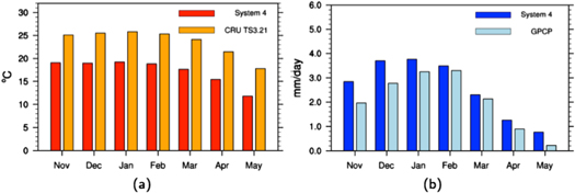
Figure 1. Botswana monthly (a) temperature and (b) precipitation climatology from System 4 hindcasts and observations.
Download figure:
Standard image High-resolution imageThe spatial pattern of model and reference climatology with the associated bias is shown in figure 2, for temperature and precipitation. The field is averaged across Dec–Feb, as this is a period of the highest rainfall, associated with enhanced vector development. Figure 2(a) shows there is a positive Southeast to Northwest temperature gradient across the region in the observations, with temperature relatively constant over Botswana itself. The spatial pattern is similar in System 4 (figure 2(b)), albeit with a large cold bias of around 6 °C.
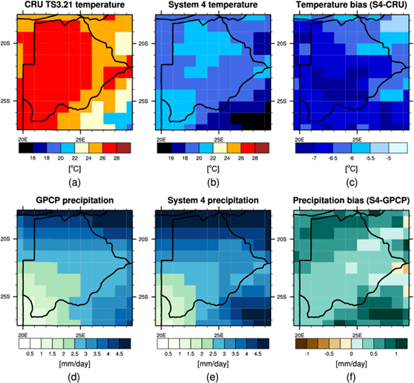
Figure 2. Top row: Dec–Jan–Feb Botswana climatology maps for 2 m air temperature for (a) CRU observations, (b) System 4, November start dates and (c) the corresponding temperature bias of System 4. Bottom row: precipitation climatology for (d) GPCP observations, (e) System 4 and (f) the corresponding precipitation bias.
Download figure:
Standard image High-resolution imageThe precipitation pattern from GPCP shows a minimum in the South East of the region, with maxima in the North and Southeast (figure 2(d)). System 4 reproduces the pattern well (figure 2(e)), with a spatially heterogeneous wet bias. Overall the model is around 0.5 mm d−1 too wet, whilst in the climatologically wettest regions it is around twice this.
Forecast skill for the climatic drivers is shown in figure 3, with plots of the ROC area for forecasts for UT and LT Dec–Feb temperature and precipitation events. Temperature forecast skill is significant at the 95% level for both UT and LT events, for most of the region. Skill is lower for precipitation, however a large part of the region exhibits skill above significance.

Figure 3. Maps of the Relative Operating Characteristic area under curve for UT (a), (b) and LT (c), (d) Dec–Jan–Feb (DJF) average temperature (a), (c) and precipitation (b), (d), from System 4 forecasts initialized at the start of November. Validation targets are CRU and GPCP data, respectively, and the cross-hatching indicates where the score is significant above the 95% level.
Download figure:
Standard image High-resolution image3.2. Validation of the malaria output
The output of the seasonal hindcasts driven through the LMM is shown in figure 4, which shows the time-averaged incidence for Botswana for each month of the forecast. The large cold bias has been corrected following the method described in the methodology; without this correction the simulated malaria is effectively zero (not shown). This is expected as the uncalibrated temperatures generally remain below the sporogonic temperature threshold (18 °C), preventing parasite development within the mosquito vector as simulated by the model.

Figure 4. Cases of malaria incidence per 100 people output by the LMM after temperature bias correction for both the raw and the seamless calibrated forecast system averaged over Botswana, averaged across all forecast start dates. Only the time period simulated by the forecast (i.e. seven months from the start of November) is shown.
Download figure:
Standard image High-resolution imageWith the bias correction the incidence follows a cycle peaking in March, with some slight difference in the raw System 4 and the seamless runs; seamless runs show a slight decrease in simulated malaria incidence during March and April. However this difference is not large with respect to the magnitude of the averaged monthly incidence.
Figure 5 shows the explicit forecast probabilities for upper and lower tercile (UT and LT) events across the hindcast period, along with the occurrence or non-occurrence of events according to the observed malaria data. The baseline frequency of the event (in the case of tercile events this is one third) is used as a decision threshold, and plotted as a red line on the figure. This can then be used to calculate some forecast statistics:'hits', 'misses', 'false alarms' and 'correct rejections'. From this one can compare the total number of correct ('hits' and 'correct rejections') to the number of incorrect forecasts ('misses' and 'false alarms'). These statistics are dependent on the decision threshold, which can be calibrated based on the hindcasts to maximize forecast value, and would likely take a different value for different events. However here the decision threshold is left uncalibrated; we use the climatological frequency of a tercile event (i.e. 33%) as a threshold, for demonstrative purposes. Using this frequency as a threshold represents the case where a warning is issued when the issued model probability is higher a climatological forecast (since a climatological forecast for a tercile event is always 33%).
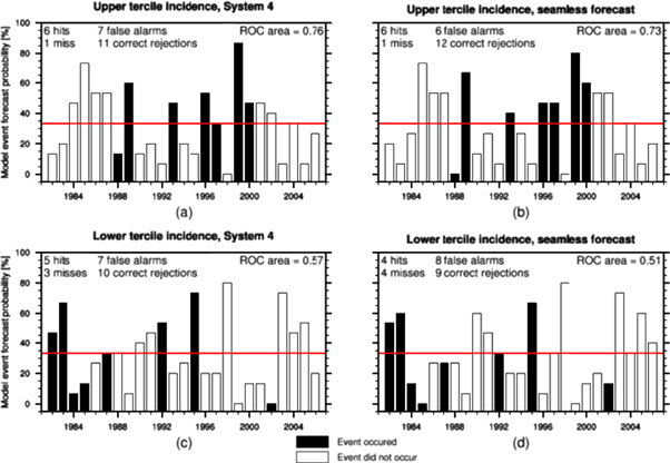
Figure 5. Malaria incidence forecast probabilities over the hindcast period for UT (a), (b) and LT (c), (d) incidence. The bar height indicates the event probability forecast by the model, black bars indicate the occurrence of the event in the observational data and white bars correspond to years where the event did not occur. Results are shown for (a), (c) the calibrated System 4 forecasts and (b), (d) the 'seamless' system. The red line indicates the baseline frequency of events, which is used here as a warning threshold, allowing calculation of performance statistics.
Download figure:
Standard image High-resolution imageBefore temperature biases have been corrected, the skill is low for both UT and LT event forecasts, for both the raw System 4 and seamless systems: in all instances the number of incorrect years is larger than the number of correctly forecast years (not shown). The ROC area for the uncorrected hindcasts is also well below 95% significance. With bias correction the skill is much improved (figure 5). For the forecasts of LT events, ROC area is still below significance, and the number of correct and incorrect years is roughly equal. However, the ROC area for UT forecasts is around the 95% significance level for the raw System 4 and the seamless calibrated system (0.76 and 0.73 respectively). For the raw and calibrated systems, using the baseline frequency as a decision threshold results in six out of seven UT years correctly forecast.
Skill as measured by the ROC area is summarized in table 1. This also includes results from previous work, where seasonal hindcasts from the ENSEMBLES project (Weisheimer et al 2009) were used to drive the LMM. This shows the result where the LMM was driven by both the multi-model ENSEMBLES system and by the previously ECMWF model, System 3, alone. These results are previously unpublished and not directly comparable, as the ENSEMBLES simulations were only carried out for the period 1982–2001. In all cases, results are improved by bias correction, with the single model System 4 hindcasts showing the best result for UT forecasts of malaria incidence, beating the multi-model forecasting system. For LT events, the ENSEMBLES multi-model system shows the highest score, which is not matched by System 4.
Table 1. ROC area for UT and LT malaria incidence forecasts, including previous work with the ENSEMBLES hindcast data. The scores are shown for simulations where the temperature input has been bias-corrected. Asterisks indicate where score is significant at the 95% level, and bold numbers indicate the system with the highest score for each event (N.B. The ENSEMBLES period is different from the System 4 period, finishing in 2001 rather than 2006).
| Hindcast data | UT | LT |
|---|---|---|
| System 4 | 0.76* | 0.57 |
| System 4 (seamless) | 0.73 | 0.51 |
| ENSEMBLES (System 3) | 0.59 | 0.81* |
| ENSEMBLES (multi-model) | 0.69 | 0.85* |
3.3. Investigating the source of forecast error
It is clear from figure 5 that the forecast is imperfect, and that there is a tendency for false alarms (at least when using a climatological decision threshold). This is in part likely due to a low signal-noise ratio; in seasonal climate predictions the ratio of the predictable signal generally decreases from forecast initialization (e.g. Misra and Li 2014), with a short-lead forecast giving a clearer signal than one for conditions many months in advance. In the current system the malaria model is driven by a climate forecast up to seven months ahead; a low signal to noise ratio can be expected. The highest signal-noise ratio and skill is generally expected for large-scale spatial average (e.g. global, hemispheric or continental), with lower signal-noise ratio and skill expected for smaller regional domains (e.g. Masson and Knutti 2011, MacLeod et al 2012), as in the current case. Furthermore, precipitation is a particularly noisy variable in climate models (e.g. Hawkins and Sutton 2011); using this to drive another model further suggests that one should not be surprised by noisy output.
Despite a low signal-noise ratio, we make some attempt here to answer the question: why does the forecast occasionally get it wrong? We do this by considering whether the temperature and precipitation forecasts driving 'good' and 'bad' malaria forecasts share any corresponding features. These driving climate forecasts are plotted in figure 6, which shows the distribution of the ensemble of standardized DJF temperature and precipitation anomalies for each validation year. The forecast is noisy but has some skill: of all 25 years the 5–95 percentile range of the ensemble contains the observation in all but three years for temperature, and four for precipitation.
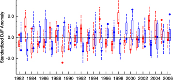
Figure 6. Ensemble forecast of DJF temperature (red) and precipitation (blue), for each year of the validation period. The year labeling corresponds to figure 5 (for example, the DJF 1982 forecast is initialized in November 1981 and gives a prediction of malaria incidence for 1982). Boxes indicate the interquartile range and median of the ensemble, whilst the whiskers represent the 5th and 95th percentiles. Observations from CRU and GPCP are represented by dots.
Download figure:
Standard image High-resolution imageDue to the non-linear relationship between these variables and resultant incidence it is not easy to draw clear conclusions of cause and effect between large-scale averages; there is uncertainty in the relationship between seasonal average climate and malaria risk (MacLeod and Morse 2014). However upon scrutiny of figures 5 and 6, two observations present themselves:
- Years when the median of the precipitation forecast is positive and the observation is negative (i.e. over prediction of rainfall) tend to over predict malaria incidence and result in false alarms of UT incidence. These years correspond to 1984, 1985, 1986, 1999, 2001 and 2002: all are UT false alarms in figure 5(a) (except for 1999, which is an UT hit).
- Forecasts of large positive temperature anomalies tend to result in high probabilities of LT malaria incidence. For example, the years with the largest predicted positive temperature anomalies correspond to 1983, 1992, 1995, 1998, 2003 and 2004. Of these, five give probabilities of LT incidence greater than 50% (2004 has a probability of 47%). Furthermore for all years with LT incidence probability below 20% (1984, 1985, 1999, 2000, 2001 and 2002) the corresponding temperature forecast has a negative median anomaly.
Enhanced precipitation creates breeding grounds for mosquitos, and too high temperature reduces the vector survival, this is consistent with previous studies of the climate–malaria relationship in the region (Thomson et al 2006).
The second relationship is also supported by the observations and related modeling assumptions: mosquito survival rate drops off at temperatures greater than 30 °C (Martens et al 1997, Hoshen and Morse 2004, Kirby and Lindsay 2009). Considering that the average DJF temperature in Botswana is around 26 °C (figures 1 and 2), positive anomalies relative to this mean are likely to pass the threshold above which mosquito survival drops off. Negative anomalies relative to this mean would still have a high survival rate and it would require a rather large negative anomaly for incidence to be severely affected, when temperatures drop below the 18 °C sporogonic threshold.
These statements should be taken as preliminary hypotheses, further in-depth analysis is necessary to understand the true pathways of cause-and effect. For example, further work might consider the characteristics of the driving forecast outside of the rainy season, the impact of intra-seasonal variability in the temperature and precipitation time series and the temporal evolution of the full suite of output from the malaria model (MacLeod and Morse 2014).
To investigate further the impact of an imperfect driving seasonal forecast, we perform additional simulations where the LMM is driven by temperature and precipitation from the ERA-Interim reanalysis, assumed here to represent the observed meteorological conditions (the lack of gridded daily data observation for the region necessitates the use of reanalysis). Results from this simulation are shown in figure 7, where the result from the ERA-I driven simulation is shown alongside the observed incidence and the forecasted ensemble of the LMM driven by the System 4 data. The incidence simulated by ERA-LMM can be interpreted as being the best that the LMM can do, as if it had perfect driving climatic conditions. In the situation where observed incidence is not reproduced by either the ERA-LMM or the System 4-LMM estimates, it is possible that the situation is such that model would be unable to make a good incidence forecast even with perfect input climate forecast data (i.e. if the climate state was exactly known). Alternatively it may be the case that other external factors were active in those years that impacted the resultant observed incidence (e.g. a short term control intervention). This situation is observed for the 1987, 1996, 1998 and 2002 hindcast years.

Figure 7. As figure 6, for System 4 JFMAM malaria incidence. Dots indicate observed malaria incidence, whilst the crosses indicate the incidence simulated by the LMM driven by ERA-Interim reanalysis.
Download figure:
Standard image High-resolution image
Years where all three elements of figure 7 match up can be tentatively interpreted as good driving conditions, transformed accurately into an accurate malaria forecast. This is the case for 1983, 1986, 1989–1995, 1997, 1999, 2001 and 2003–2005. Of the remaining years, 1982, 1984 and 1985 suggest that a good forecast may be possible had the seasonal climate forecast been better, whilst 2000 and 2006 indicate that the malaria ensemble forecast captures well the observed incidence, whilst the 'perfect' ERAI-LMM is well outside the range. This suggests that either System 4 for those years is closer to reality than the reanalysis, or that there is some error cancellation occurring when seasonal forecast temperature and rainfall are integrated by the LMM, leading to the right answer, but for the wrong reasons. These years show good temperature forecasts, with an under prediction of precipitation (figure 6): this does not support the hypothesis that the climate forecast (at least for precipitation) is better than the reanalysis for these years.
4. Discussion and conclusions
We have demonstrated the potential for producing skillful forecasts of anomalously high malaria seasons over Botswana, months in advance. The skill assessment is based on the hindcasts produced by an operational seasonal forecast system and therefore a forecast that could be issued to users immediately. Probabilistic information about the risk of an anomalously high risk upcoming malaria season, whilst imperfect, could provide significant benefits through advanced and targeted allocation of resources for malaria control.
Temperature bias correction of the forecast is vital: system 4 is 6 °C too cold over Botswana and the bias correction greatly improves the skill of forecasts. This is somewhat expected, as the temperature climatology is above the sporogonic threshold of 18 °C: without the bias correction, development of the parasite within the vector in the model is inhibited and malaria transmission does not occur. This is reflected in the low incidence output from the model. The temperature bias correction method employed here is relatively simple and perhaps a more sophisticated method would improve skill further, such as one which preserves any co-variation between the temperature and precipitation time series (Piani and Haerter 2012).
The seamless calibrated system (which differs from the System 4 hindcasts only in the first four weeks) does not apparently improve the malaria forecasts. Since most production of malaria occurs during and after the main rainy season, it is perhaps not surprising that modifying the input ahead of this period makes little difference. Furthermore, the System 4 precipitation bias over Botswana is small, so calibrated rainfall makes little impact. It may be the case that in regions where the precipitation biases are large this calibrated rainfall dataset may improve the malaria forecasts, however here it does not. However, the average malaria is taken over a much longer time period than the calibration period of the seamless forecast; an extended calibration may have more impact.
The skill demonstrated here is likely an underestimate of the operational skill of the forecast. It has been shown that using smaller ensembles underestimates forecast skill (Richardson 2000) and the operational System 4 forecast runs with a much larger ensemble than the hindcast studied here (51 rather than 15 members). Ideally skill would be estimated from a hindcast with an ensemble of comparable size to the operational forecast, however in reality this is not possible due to computing constraints—generally the model is upgraded before sufficient operational forecasts have been archived. Forecasts may be improved further by using a multi-model ensemble of state-of-the-art climate models such as the operational EUROSIP project (Vitart et al 2007); it has been shown that multi-model techniques improve forecast skill and reliability beyond that of any constituent single model (Hagedorn et al 2005). Furthermore an operational malaria early warning system would not only rely on one forecast made months in advance, but each year as the malaria season approaches it would be able to utilize updated shorter-term forecasts and climate observations, refining the forecast of expected incidence.
Since statistical forecasts between seasonal precipitation forecasts and malaria have been shown to have a good fit with incidence observations (Thomson et al 2006), Occam's razor suggests that this more complex dynamical modeling system is unnecessary. However this is not the case. Statistical approaches are based on a fit to a historical period; the validity of a statistical model outside of this period requires the relationship between a set of predictors and the modeled outcome is preserved in the new situation. That is, for a statistical malaria–climate model to be useful, it requires the empirical relationship between precipitation and malaria incidence to be unchanged into the future. Considering the nonlinear relationship between temperature, rainfall and malaria incidence, and the projected 21st century changes in temperature and rainfall, it is likely that statistical methods are somewhat compromised under climate change. A dynamical process-based approach is not as limited by a non-stationary system as a statistical model is and there is more potential for its use in a changing future.
Whilst the malaria incidence dataset employed for model validation is the longest yet used to quantify the skill of such a climate-driven disease prediction on seasonal timescales, it has some limitations. The first is that there is only one data point for each year, which does not allow estimation of the skill in predicting the onset and seasonal timing of epidemics. Secondly, as the incidence data corresponds to a large spatial average, it is not possible to estimate the skill of seasonal predictions at a sub-national scale. However despite the limitations of the dataset, a nationwide annual malaria warning based on seasonal climate forecasts has the potential to be useful for guiding public health interventions in Botswana.
Interventions have continued in Botswana, from DDT spraying in the 1950s to the current program of bed net distribution, indoor residual spraying and winter biolarviciding, alongside passive surveillance (Chihanga et al 2013). Incidence forecasts can contribute to the surveillance program and guide the allocation of financial and material resources. For example, based on a forecast issued in November for UT malaria for the following year, the government or an NGO working in the area may decide to divert funding from other projects to distribute extra bed nets, or provide extra resources for indoor spraying, reducing the harm from a particularly virulent season.
Successful intervention programs themselves provide further challenges for seasonal malaria forecasting. In this current work, though incidence anomalies have been corrected for major policy intervention post-1996 (Thomson et al 2006), the model does not take into account non-climate factors, meaning that the modeling system predicts malaria incidence only in the absence of any intervention. A real-time forecast of a high malaria event that triggers an intervention may be undermined by that very action; if the intervention works then high incidence is avoided and the forecast appears wrong. Despite this, a forecasted suitability for high incidence may still be observable indirectly, for example by monitoring the level of parasite and mosquito numbers.
Another concern related to the use of forecasts is that different forecast users likely have different sensitivities to false alarms and/or misses; an imperfect forecast system is not necessarily useful for every user. For example, a user who can act at a cost of £800 to prevent loss of £1000 would find little use in a system which forecasts every event but has many false alarms, whilst a user with the same value of loss but who can act with a cost of £200 may find use in this system. To some extent it is possible to tune the forecast system for a particular value of cost/loss by varying the decision threshold (for example by calibrating against potential economic value, see Joliffe and Stephenson (2003)). However imperfection cannot be avoided and incorrect forecasts are likely to remain a feature of seasonal forecasting systems for the foreseeable future.
It is also worth concluding with a further note of caution related to incorrect forecasts. Because each forecasted season is separated by a year, it is quite possible that an operational forecast that is skillful overall will cluster imperfect forecasts. For example, in the UT incidence forecasts for System 4 (figure 5(a)), the forecast for every year between 1980 and 1984 would have been a false alarm, followed by a miss in 1985. Following this, the system forecasts successfully every year until 2001—similar to the story of 'the boy who cried wolf' (see also, Roulston and Smith 2004). With hindsight it is clear that there is skill in the system, however a decision-maker at the start of 1986 would understandably have low confidence in the model. Considering the timescales on which governments, NGOs and health services might fund a health early warning system, alongside their competing priorities, it is quite possible that a forecasting system issuing an incorrect forecast five years in a row would be thrown out on the sixth—even though in the long run it may prove its worth. It is therefore vital that forecast providers are absolutely transparent with this possibility and proactively communicate it with users, to prevent a string of bad luck diminishing the long-term positive impact of the forecast. Indeed, a close analysis of the reasons behind incorrect forecast such as that carried out here can further increase the use of the forecasting system, as it may allow an a priori indication that a forecast may turn out to be a bust. This is yet another reason to work across interdisciplinary boundaries, so that knowledge can be successfully and effectively transferred from centers of research to decision-making institutions.
Acknowledgments
The authors would like to jointly thank Madeline Thomson (IRI) for providing the extended Botswana dataset, as well as the anonymous reviewers, whose comments helped improve the manuscript. DM recognizes support from NERC for a PhD stipend (grant number NE/H524757/1). APM, AJ, CC and FD-G were jointly funded by the European Union FP7 projects Quantifying Weather and Climate Impacts on Health in Developing Countries (QWeCI, grant agreement number 243964) and HEALTHY FUTURES (grant agreement 266327). CC and APM also acknowledge funding support from the End-to-End Quantification of Uncertainty for Impacts Prediction (EQUIP) Natural Environmental Research Council Project NE/H003487/1.
Conflict of intrest
The authors declare no competing financial interests.