


Abstract
• Background and Aims DNA flow cytometry requires preparation of suspensions of intact nuclei, which are stained using a DNA-specific fluorochrome prior to analysis. Various buffer formulas were developed to preserve nuclear integrity, protect DNA from degradation and facilitate its stoichiometric staining. Although nuclear isolation buffers differ considerably in chemical composition, no systematic comparison of their performance has been made until now. This knowledge is required to select the appropriate buffer for a given species and tissue.
• Methods Four common lysis buffers (Galbraith's, LB01, Otto's and Tris.MgCl2) were used to prepare samples from leaf tissues of seven plant species (Sedum burrito, Oxalis pes-caprae, Lycopersicon esculentum, Celtis australis, Pisum sativum, Festuca rothmaleri and Vicia faba). The species were selected to cover a wide range of genome sizes (1·30–26·90 pg per 2C DNA) and a variety of leaf tissue types. The following parameters were assessed: forward (FS) and side (SS) light scatters, fluorescence of propidium iodide-stained nuclei, coefficient of variation of DNA peaks, presence of debris background and the number of nuclei released from sample tissue. The experiments were performed independently by two operators and repeated on three different days.
• Key Results Clear differences among buffers were observed. With the exception of O. pes-caprae, any buffer provided acceptable results for all species. LB01 and Otto's were generally the best buffers, with Otto's buffer providing better results in species with low DNA content. Galbraith's buffer led to satisfactory results and Tris.MgCl2 was generally the worst, although it yielded the best histograms in C. australis. A combined analysis of FS and SS provided a ‘fingerprint’ for each buffer. The variation between days was more significant than the variation between operators.
• Conclusions Each lysis buffer tested responded to a specific problem differently and none of the buffers worked best with all species. These results expand our knowledge on nuclear isolation buffers and will facilitate selection of the most appropriate buffer depending on species, tissue type and the presence of cytosolic compounds interfering with DNA staining.
INTRODUCTION
Flow cytometry (FCM) was developed in the 1950s but its application to plant sciences was delayed until the late 1980s when it became an important technique for estimation of nuclear DNA content, determination of DNA ploidy level and cell cycle analysis (Galbraith, 2004; Shapiro, 2004; Bennett and Leitch, 2005). This delay was mainly due to problems with the preparation of suspensions of intact nuclei from thick tissues consisting of cells with a rigid cell wall. In his pioneering work, Heller (1973) used hydrolytic enzymes to digest cell walls and release nuclei from fixed tissues. The method was time consuming and rarely followed by others. Among later investigators, Ulrich and Ulrich (1986), Ulrich et al. (1988) and Bergounioux et al. (1988, 1992) employed a modified approach in which cell nuclei were released after hypotonic lysis of intact protoplasts. In addition to being time consuming, the need for intact protoplasts limited the application of this protocol to some species and certain types of tissues. As an alternative, Galbraith et al. (1983) developed a rapid and convenient method for isolation of plant nuclei by chopping plant tissues in a lysis buffer. Since then, this has been the main and most reliable method for nuclear isolation in plant FCM.
In addition to releasing nuclei from intact cells, lysis buffers must ensure the stability of nuclei throughout the experiment, protect DNA from degradation and facilitate stoichiometric staining. Since the late 1980s, some laboratories have developed their own buffer formulas. As a result, about 25 different lysis buffers are known, although only eight are commonly used. Their chemical composition varies, but it usually includes chromatin stabilizers (e.g. MgCl2, MgSO4, spermine); chelator agents [e.g. ethylenediaminetetraacetic acid (EDTA), sodium citrate] to bind divalent cations, which serve as nuclease cofactors; inorganic salts (e.g. KCl, NaCl) to achieve proper ionic strength; organic buffers [e.g. 3-(N-morpholino) propanesulfonic acid (MOPS), Tris-(hydroxymethyl)-aminomethane (Tris) and 4-(hydroxymethyl)piperazine-1-ethanesulfonic acid (HEPES)] to stabilize the pH of the solution (usually set between 7·0 and 8·0); and non-ionic detergents (e.g. Triton X-100, Tween 20) to release nuclei, disrupt chloroplasts as fluorescent entities, remove and hinder cytoplasmatic remnants from nuclei surface, and decrease the aggregation affinity of nuclei and debris (Coba de la Peña and Brown, 2001; Doležel and Bartoš, 2005).
Given the different chemical composition and diversity of plant tissues, it may be expected that each buffer would perform differently. This problem was exacerbated by the recent observation of the presence of cytosolic compounds that are released during nuclei isolation. These compounds interact with nuclear DNA and/or the fluorochrome, affecting sample quality and causing stoichiometric errors in DNA staining (Noirot et al., 2000, 2003; Pinto et al., 2004; Loureiro et al., 2006; Walker et al., 2006). Loureiro et al. (2006) observed that nuclei of Pisum sativum and Zea mays responded differently to tannic acid, a common phenolic compound in plants, when isolated in different nuclear isolation buffers. However, no systematic comparison of lysis buffers has been made until now.
We set out to compare four of the most common buffers that differ in chemical composition: Galbraith's buffer (Galbraith et al., 1983), LB01 (Doležel et al., 1989), Otto's buffer (Otto, 1992; Doležel and Göhde, 1995) and Tris.MgCl2 (Pfosser et al., 1995). We evaluated light scatter and fluorescence properties of nuclei in suspension, the presence of debris background and the number of nuclei released from sample tissue. Samples were prepared from leaf tissue of seven plant species that cover a wide range of genome sizes (1·30–26·90 pg per 2C DNA) and whose tissues differ in structure and chemical composition (Table 1). Pisum sativum, Lycopersicon esculentum and Vicia faba are common DNA reference standards for FCM; Sedum burrito, a species from Crassulaceae, has fleshy leaves with many reserve substances; Oxalis pes-caprae has an acidic cell sap (Castro et al., 2005); Celtis australis releases mucilaginous compounds after tissue homogenization (Rodriguez et al., 2005a); and Festuca rothmaleri has rigid leaves that are difficult to chop. The effect of instrumental drift and operator were also evaluated. The main goal of the study was to provide data that facilitate selection of the appropriate buffer and to propose strategies to minimize common problems in plant DNA flow cytometry.
Nuclear DNA content of the seven plant species used in this study
| Species | Family | Nuclear DNA content (pg per 2C) | Reference |
|---|---|---|---|
| Sedum burrito | Crassulaceae | 1·30 | This work |
| Oxalis pes-caprae | Oxalidaceae | 1·37 | Castro et al. (2005) |
| Lycopersicon esculentum ‘Stupické’ | Solanaceae | 1·96 | Doležel et al. (1992) |
| Celtis australis | Ulmaceae | 2·46 | Rodriguez et al. (2005a) |
| Pisum sativum ‘Ctirad’ | Fabaceae | 9·09 | Doležel et al. (1989) |
| Festuca rothmaleri | Poaceae | 13·67 | J. Loureiro (unpubl. data) |
| Vicia faba ‘Inovec’ | Fabaceae | 26·90 | Doležel et al. (1992) |
MATERIALS AND METHODS
Plant material
Plants of Lycopersicon esculentum ‘Stupické’ (Solanaceae), Pisum sativum ‘Ctirad’ (Fabaceae) and Vicia faba ‘Inovec’ (Fabaceae) were grown from seeds. Plants of Festuca rothmaleri (Poaceae) and Oxalis pes-caprae (Oxalidaceae) were kindly provided by Prof. Paulo Silveira and Dr Sílvia Castro (Department of Biology, University of Aveiro, Portugal), respectively. Plants of Sedum burrito (Crassulaceae) were obtained from Flôr do Centro Horticultural Centre (Mira, Portugal). All plants were maintained in a greenhouse at 22 ± 2 °C, with a photoperiod of 16 h and a light intensity of 530 ± 2 μmol m−2 s−1. Leaves of Celtis australis (Ulmaceae) were collected directly from field-growing trees in Aveiro, Portugal.
Sample preparation
Approximately 40–50 mg of young leaf tissue was used for sample preparation. The amount of material required to release a sufficient number of nuclei in S. burrito had to be increased to approximately 500 mg due to the fleshy nature of the leaves. Nuclei suspensions were prepared according to Galbraith et al. (1983). Four common nuclear isolation buffers (Doležel and Bartoš, 2005) were used to prepare samples (Table 2). One millilitre of nuclei suspension was recovered and filtered through a 50-µm nylon filter to remove cell fragments and large debris. Nuclei were stained with 50 µg mL−1 propidium iodide (PI) (Fluka, Buchs, Switzerland), and 50 µg mL−1 RNase (Sigma, St Louis, MO, USA) was added to the nuclear suspension to prevent staining of double-stranded RNA. Samples were incubated on ice and analysed within 10 min.
Four nuclear isolation buffers most frequently used in plant DNA flow cytometry
| Buffer | Composition* | Reference |
|---|---|---|
| Galbraith | 45 mm MgCl2, 30 mm sodium citrate, 20 mm MOPS, 0·1 % (v/v) Triton X-100, pH 7·0 | Galbraith et al. (1983) |
| LB01 | 15 mM Tris, 2 mm Na2EDTA, 0·5 mm spermine.4HCl, 80 mm KCl, 20 mm NaCl, 0·1 % (v/v) Triton X-100, pH 8·0† | Doležel et al. (1989) |
| Otto‡ | Otto I: 100 mm citric acid, 0·5 % (v/v) Tween 20 (pH 2–3) Otto II: 400 mm Na2PO4·12H2O (pH 8–9) | Otto (1992), Doležel and Göhde (1995) |
| Tris.MgCl2 | 200 mm Tris, 4 mm MgCl2.6H2O, 0·5 % (v/v) Triton X-100, pH 7·5 | Pfosser et al. (1995) |
Final concentrations are given.
The buffer formula contains 15 mm mercaptoethanol. However, as the other buffers were used without additives that suppress the negative effect of phenols and other cytosolic compounds, LB01 was used without mercaptoethanol.
pH of the buffers is not adjusted. The nuclei are isolated in Otto I buffer; DNA staining is done in a mixture of Otto I and Otto II (1 : 2) with a final volume of 1 mL.
Flow cytometric analyses
Samples were analysed in a Coulter EPICS XL (Coulter Electronics, Hialeah, FL, USA) flow cytometer equipped with an air-cooled argon-ion laser tuned at 15 mW and operating at 488 nm. Fluorescence was collected through a 645-nm dichroic long-pass filter and a 620-nm band-pass filter. The results were acquired using the SYSTEM II software version 3·0 (Coulter Electronics). Prior to analysis, the instrument was checked for linearity with fluorescent beads (Coulter Electronics), and the amplification settings were kept constant throughout the experiment.
The following parameters were evaluated in each sample: forward light scatter (FS, to estimate relative size of particles), side light scatter (SS, to estimate relative optical complexity of particles), relative fluorescence intensity of PI-stained nuclei (FL), half peak coefficient of variation (CV) of the G0/G1 peak (to estimate nuclei integrity and variation in DNA staining), a debris background factor (DF, to assess sample quality) and a nuclear yield factor (YF, to compare the amount of nuclei in suspension independently of the amount of leaf tissue used).
The analysis was performed on three different days and by two operators (labelled here as A and B). Five replicates were performed per operator for each buffer and in each replicate at least 5000 nuclei were analysed. Histograms of FL obtained with the best and worst performing buffers were overlaid using WinMDI software (Trotter, 2000) (Fig. 1).
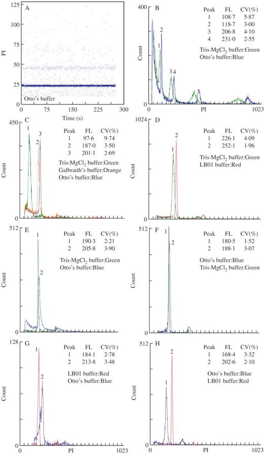
Cytogram of fluorescence intensity (PI, relative channel numbers) vs. time of Pisum sativum nuclei isolated with Otto's buffer (A) and histograms of relative fluorescence intensities (B–H), which show overlays of distributions obtained with the best and worst performing buffer for each species: (B) Sedum burrito, (C) Oxalis pes-caprae, (D) Lycopersicon esculentum, (E) Celtis australis, (F) Pisum sativum, (G) Festuca rothmaleri and (H) Vicia faba. Relative mean channel numbers and coefficients of variation (CV, %) of G0/G1 peaks are given. Four lysis buffers were compared: LB01 (red), Galbraith's (orange), Tris.MgCl2 (green) and Otto's (blue).
Statistical analyses
Statistical analyses were performed using a three-way ANOVA (SigmaStat for Windows version 3·11) to assess for differences among buffers and dates and between operators. When treatments were significantly different, a Holm–Sidak multiple comparison test was used for pair-wise comparison. Hierarchical cluster analyses were performed using NCSS 2004 (Hintze, 2004). Dendrograms highlighting dissimilarities among buffers and between operators were obtained using FS, SS, FL, CV, BF and YF. The Unweighted Pair Group Method with Arithmetic mean (UPGMA) was followed in each species as it yielded the highest co-phenetic correlation coefficient.
RESULTS
With the exception of O. pes-caprae, for which measurable samples were only obtained with Otto's and Galbraith's buffers, all buffers yielded acceptable histograms with all species tested. In any analysis, it was possible to isolate a reasonable number of nuclei (approximately 20–60 nuclei per second in a low-speed configuration), and obtain well-defined histograms with DNA peaks with acceptable CV values (<5·0 %, Galbraith et al., 2002; Fig. 1, Table 3). Table 3 indicates the best performing buffer(s) for each species. The selection criteria were the highest FL and YF values, and the lowest CV and DF values.
Flow cytometric parameters assessed in each species
| FS (channel units) | SS (channel units) | FL (channel units) | CV (%) | BF (%) | YF (nuclei s−1 mg−1) | ||||||||||||||
|---|---|---|---|---|---|---|---|---|---|---|---|---|---|---|---|---|---|---|---|
| Species | Buffer | Mean | SD | Mean | SD | Mean | SD | Mean | SD | Mean | SD | Mean | SD | ||||||
| Sedum burrito | LB01 | 57.66a | 8·724 | 11·37a | 2·448 | 110·9a | 5·93 | 4·48a | 0·407 | 69·15a | 24·903 | 0·06a | 0·004 | ||||||
| Galbraith | 41·06b | 5·171 | 5·36b | 2·299 | 112·1a | 2·57 | 3·59ab | 0·396 | 60·02a | 16·631 | 0·05b | 0·004 | |||||||
| Tris.MgCl2 | 57.50a | 8·556 | 13·34a | 2·670 | 103·0b | 6·19 | 5·61c | 1·000 | 68·85a | 13·874 | 0·05ab | 0·004 | |||||||
| Otto | 8·01c | 2·179 | 2·58c | 0·787 | 121·4c | 3·93 | 3·27b | 0·288 | 65·96a | 6·33 | 0·05ab | 0·006 | |||||||
| Oxalis pes-caprae | LB01 | – | – | – | – | – | – | – | – | – | – | – | – | ||||||
| Galbraith | 171·33a | 36·404 | 19·75a | 6·920 | 178·5a | 5·21 | 4·14a | 0·778 | 7·05a | 4·977 | 1·01a | 0·364 | |||||||
| Tris.MgCl2 | – | – | – | – | – | – | – | – | – | – | – | – | |||||||
| Otto | 26·32b | 4·933 | 3·90b | 0·641 | 200·7b | 6·24 | 3·03b | 0·415 | 8·96a | 5·908 | 0·62b | 0·125 | |||||||
| Lycopersicon esculentum | LB01 | 15·42a | 2·125 | 2·97a | 0·494 | 257·9a | 11·50 | 2·88a | 0·880 | 21·21a | 14·137 | 2·47a | 1·512 | ||||||
| Galbraith | 21·53b | 3·752 | 3·40a | 0·713 | 208·5b | 49·61 | 2·87a | 0·712 | 16·87a | 10·036 | 1·69ab | 0·814 | |||||||
| Tris.MgCl2 | 17·48a | 4·970 | 4·76b | 1·562 | 216·7b | 27·27 | 3·70b | 0·836 | 20·52a | 12·918 | 1·72ab | 1·745 | |||||||
| Otto | 3·68c | 1·537 | 1·95c | 0·766 | 269·9a | 11·17 | 2·18c | 0·266 | 28·49b | 13·254 | 0·91b | 0·617 | |||||||
| Celtis australis | LB01 | 28·47a | 4·847 | 11·45a | 3·481 | 182·1a | 13·13 | 3·02a | 0·315 | 7·66a | 3·565 | 0·50a | 0·224 | ||||||
| Galbraith | 25·57a | 1·842 | 4·54b | 0·637 | 171·3b | 7·76 | 2·87a | 0·259 | 8·27a | 3·445 | 0·35a | 0·162 | |||||||
| Tris.MgCl2 | 41·71b | 6·944 | 16·08c | 2·157 | 180·3a | 10·44 | 2·85a | 0·419 | 9·10b | 5·085 | 0·49a | 0·291 | |||||||
| Otto | 8·20c | 1·404 | 7·25b | 1·787 | 192·8c | 8·23 | 3·46b | 0·405 | 23·96c | 4·615 | 0·49a | 0·200 | |||||||
| Pisum sativum | LB01 | 47·54a | 1·550 | 10·87a | 3·078 | 183·5a | 5·06 | 2·81a | 0·461 | 7·19a | 2·823 | 2·33a | 0·490 | ||||||
| Galbraith | 51·97a | 3·624 | 5·29b | 1·155 | 178·6a | 3·36 | 3·02ab | 0·465 | 6·34a | 1·765 | 2·30a | 0·876 | |||||||
| Tris.MgCl2 | 59·37b | 4·826 | 16·74c | 2·914 | 177·7a | 11·86 | 3·29b | 0·515 | 6·39a | 2·781 | 2·59a | 0·894 | |||||||
| Otto | 5·72c | 0·993 | 4·79b | 1·083 | 190·1a | 6·06 | 1·94c | 0·180 | 9·85b | 2·668 | 1·15b | 0·367 | |||||||
| Festuca rothmaleri | LB01 | 57·35a | 1·825 | 8·57a | 0·799 | 196·1a | 6·07 | 3·24a | 0·452 | 14·23ab | 3·283 | 0·42a | 0·182 | ||||||
| Galbraith | 61·03a | 2·250 | 6·84b | 0·649 | 182·7b | 7·15 | 3·33ab | 0·459 | 15·07a | 1·974 | 0·27b | 0·131 | |||||||
| Tris.MgCl2 | 69·85a | 1·603 | 17·72c | 0·815 | 185·1b | 8·06 | 3·66ab | 0·312 | 17·30b | 5·701 | 0·54a | 0·195 | |||||||
| Otto | 13·84b | 2·846 | 8·55a | 1·603 | 210·9c | 6·77 | 3·76b | 0·613 | 23·86c | 12·992 | 0·11c | 0·066 | |||||||
| Vicia faba | LB01 | 104·82a | 6·021 | 11·61a | 1·742 | 201·5a | 4·45 | 2·40a | 0·178 | 6·36a | 2·326 | 0·87a | 0·290 | ||||||
| Galbraith | 114·55b | 2·787 | 8·58b | 1·306 | 196·9a | 4·88 | 2·41a | 0·148 | 5·80a | 0·806 | 0·82a | 0·235 | |||||||
| Tris.MgCl2 | 115·45b | 5·194 | 20·36c | 1·443 | 191·5a | 9·10 | 2·91b | 0·272 | 6·85a | 4·609 | 1·30b | 0·345 | |||||||
| Otto | 21·56c | 8·721 | 14·05a | 7·589 | 184·2a | 16·92 | 2·22a | 0·532 | 4·35a | 1·751 | 0·45c | 0·18 | |||||||
Values are given as mean and standard deviation of the mean (SD) of forward scatter (FS, channel units); side scatter (SS, channel units); fluorescence (FL, channel units); coefficient of variation of G0/G1 DNA peak (CV, %); background factor (BF, %) and nuclear yield factor (YF, nuclei s−1 mg−1). Means followed by the same letter (a, b or c) are not statistically different according to the multiple comparison Holm–Sidak test at P < 0.05. Buffer(s) that performed best in each species are shown in bold type.
Sedum burrito
This species was investigated because of its expected small genome size and fleshy leaves. FCM analysis revealed the occurrence of polysomaty, as demonstrated by the presence of discrete populations of nuclei with DNA contents of 2C, 4C, 8C, 16C and higher. In order to observe a higher number of endopolyploidy levels, instrument gain was set such that the 2C peak was approximately on channel 100. The 2C nuclear DNA content was estimated as 1·30 ± 0·09 pg (2C = 1271 Mbp); this is the first estimate for this species (Table 1). Comparative analysis of the four buffers revealed that Otto's was the best in this species. In general, YF values were low (the lowest values from all the test species), whereas DF values were high (approx. 65·0 %; Table 3, Fig. 1B).
Oxalis pes-caprae
Only Otto's and Galbraith's buffers provided acceptable results with this species. Otto's was clearly and significantly better than Galbraith's (Fig. 1C), with higher mean FL intensities and lower CV values (Table 3). Figure 1C also shows the histogram obtained after nuclear isolation with Tris.MgCl2 buffer. In this case a G0/G1 peak with an unacceptable CV value (9·74 %) and considerable loss of fluorescence was obtained. A similar result was obtained for nuclei isolated with LB01.
Lycopersicon esculentum
Acceptable results were obtained with all four buffers. Two buffer groups with statistically significant differences in FL were obtained. Samples prepared with Galbraith's and Tris.MgCl2 buffers yielded lower mean FL values than their counterparts prepared with LB01 and Otto's buffers (Fig. 1D). The FL values were highly heterogeneous among buffers. Otto's and LB01 were the best buffers, with Otto's providing lower CV values and higher FL, but lower YF and higher BF than LB01 (Table 3).
Celtis australis
Low CV values (<3·0 %) and low DF (<10·0 %) were observed for this species. Nevertheless, it was not easy to obtain suffiecient nuclei and the second lowest YF values were observed in this species. With regard to FL, only LB01 and Tris.MgCl2 buffers were not statistically different, with nuclei isolated from Galbraith's buffer presenting the lowest mean FL and Otto's the highest mean FL. All parameters combined, Tris.MgCl2 and LB01 were the best buffers, as nuclei in Tris.MgCl2 presented the lowest CV values and similar FL intensity and YF values as in LB01 (Table 3, Fig. 1E).
Pisum sativum
In this species, all buffers performed reasonably well. The lowest FL intensities were obtained for nuclei isolated with Tris.MgCl2, although no statistically significant differences were observed among the tested buffers. The best buffer for this species was Otto's (Table 3, Fig. 1F). Among the investigated species, P. sativum was the one with the highest YF.
Festuca rothmaleri
With the exception of CV values and YF, overall results for this species were satisfying with all four buffers tested. No statistically significant differences were found regarding the FL of nuclei isolated in Tris.MgCl2 or Galbraith's buffers, as nuclei from both buffers presented low FL values. The best buffer for this species was LB01 (Table 3, Fig. 1G).
Vicia faba
This species gave the lowest CV and DF values among those tested. Generally, the results were very similar to those obtained for P. sativum. FL was similar for all the buffers, and no statistically significant differences were observed. Interestingly, Vicia faba was the only species for which Otto's was not the buffer with the highest FL (Fig. 1H). Despite low CV values of DNA peaks, this buffer gave the worst results, with the G0/G1 peak shifted towards the lower channels. This was due to fluorescence instability, which decreased over time. In all other species and with the remaining buffers, FL was stable after 10 min of incubation with PI (Fig. 1A). Results obtained with LB01 and Galbraith's buffers were similar and the best for this species (Table 3).
Analysis of FS and SS
Generally, FS and SS values differed considerably among the test buffers. Nevertheless, in most of the species, analysis of scatter parameters revealed that two of the four buffers were more similar than the others, and no statistically significant differences were observed between them. Interestingly, and with the exception of S. burrito, buffers that had similar FS mean values were not those that had similar SS values. This can be seen on cytograms of FS vs. SS obtained in P. sativum (Fig. 2). In this species and for FS, no statistically significant differences were observed between LB01 and Galbraith's buffers; for SS, no difference was observed for Galbraith's and Otto's buffers. Interestingly, simultaneous analysis of FS and SS resulted in a species-specific pattern that could be used as a fingerprint of each buffer.
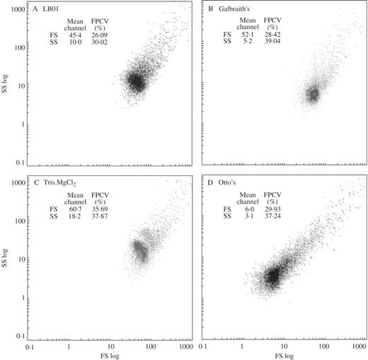
Cytograms of forward scatter (logarithmic scale, FS log) vs. side scatter (logarithmic scale, SS log) obtained after the analysis of Pisum sativum nuclei isolated with four lysis buffers: (A) LB01, (B) Galbraith's, (C) Tris.MgCl2 and (D) Otto's. The mean channel number and full peak coefficient of variation (FPCV, %) are given for both parameters. Note that the patterns of distributions are characteristic for each buffer.
Effect of operator and date of analysis
In most cases, no statistically significant differences were observed between operators and dates of analysis. Operators provided more homogeneous results than dates; in the former, statistically significant differences were observed only for BF and YF in more than one species. Significant differences between the dates of analysis were detected in some species for FS, SS, CV and BF. With regard to FL, one of the most important parameters in FCM analyses, significant among-day differences were detected only in C. australis, and differences between operators occurred only in L. esculentum. The two species more susceptible to differences were L. esculentum and V. faba (Table 4).
Three-way ANOVA analysis of the dates (D) and operators (O) for the parameters evaluated on each species
| FS | SS | FL | CV | BF | YF | |||||||||||||
|---|---|---|---|---|---|---|---|---|---|---|---|---|---|---|---|---|---|---|
| Species | D | O | D | O | D | O | D | O | D | O | D | O | ||||||
| Sedum burrito | n.s. | n.s. | n.s. | n.s. | n.s. | n.s. | n.s. | n.s. | s. | n.s. | n.s. | n.s. | ||||||
| Oxalis pes-caprae | s. | n.s. | s. | n.s. | n.s. | n.s. | s. | n.s. | n.s. | n.s. | n.s. | n.s. | ||||||
| Lycopersicon esculentum | s. | n.s. | n.s. | n.s. | n.s. | s. | s. | n.s. | s. | s. | s. | s. | ||||||
| Celtis australis | n.s. | n.s. | n.s. | n.s. | s. | n.s. | n.s. | n.s. | s. | n.s. | n.s. | n.s. | ||||||
| Pisum sativum | n.s. | n.s. | s. | n.s. | n.s. | n.s. | s. | n.s. | s. | n.s. | n.s. | n.s. | ||||||
| Festuca rothmaleri | s. | n.s. | n.s. | n.s. | n.s. | n.s. | n.s. | n.s. | n.s. | s. | n.s. | n.s. | ||||||
| Vicia faba | n.s | s. | s. | s. | n.s. | n.s. | n.s. | n.s. | n.s. | n.s. | s. | s | ||||||
Forward scatter, FS; side scatter, SS; fluorescence, FL; coefficient of variation of the G0/G1 DNA peak, CV; background factor, BF; and nuclear yield factor, YF.
n.s., not significantly different; s., significantly different at P < 0.05.
Hierarchical cluster analysis
With the exception of the results for S. burrito, the four buffers fell into two highly dissimilar and consistent clusters; one with Otto's buffer and the other with the remaining buffers. In S. burrito (Fig. 3A), one cluster was formed with Otto's and Galbraith's buffers, while the other comprised Tris.MgCl2 and LB01 buffers. In C. australis (Fig. 3C), Galbraith's buffer was more similar to LB01 and Tris.MgCl2 buffers than to Otto's buffer; in addition, ‘Tris.MgCl2 A’ was more similar to LB01 than to ‘Tris.MgCl2 B’. In P. sativum, ‘Galbraith’s A' was more related to LB01 than to ‘Galbraith’s B' (Fig. 3D), whereas for F. rothmaleri, ‘LB01 A’ was more similar to Galbraith's than to ‘LB01 B’ (Fig. 3E). In L. esculentum, two groups were formed from the second cluster: Tris.MgCl2 and ‘Galbraith A’ formed one group and LB01 and ‘Galbraith B’ formed the other (Fig. 3B). In V. faba (Fig. 3F), LB01 and Galbraith's formed one group owing to greater similarities between operators than within each buffer. As previously stated, in O. pes-caprae only two buffers (Otto's and Galbraith's) provided acceptable results, with considerable dissimilarities between them (data not shown).
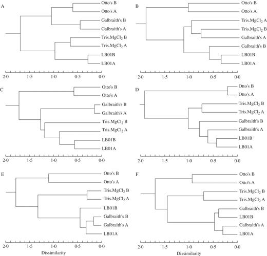
Dendrograms obtained after hierarchical cluster analysis of the following species: (A) Sedum burrito, (B) Lycopersicon esculentum, (C) Celtis australis, (D) Pisum sativum, (E) Festuca rothmaleri, (F) Vicia faba, according to the parameters FS, SS, FL, CV, BF and YF. With the exception of S. burrito, the four buffers fell into two highly dissimilar clusters of the same buffers.
DISCUSSION
Four nuclear isolation buffers were used with a set of species that were chosen to represent different types of leaf tissues and different nuclear DNA content (1·30–26·90 pg per 2C DNA). As expected, popular DNA reference standards (P. sativum, V. faba and L. esculentum) were easy to work with. Nevertheless, not all buffers worked well with L. esculentum, possibly owing to the presence of cytosolic compounds. However, as the aim of the study was to compare the performance of basic buffer formulas, the use of additives that could counteract the negative effects of cytosol was avoided.
Overall, the best results were obtained with P. sativum. As its 2C nuclear DNA content is in the middle of the known range of genome sizes in plants, this observation underlines its position as one of the best standards for plant DNA FCM. By contrast, Sedum burrito was the most difficult species to analyse due to low DNA content, occurrence of polysomaty and high leaf water content, which hampered sample preparation and analysis. Moreover, its tissues may contain tannins (J. Greilhuber, pers. comm., 2006).
In O. pes-caprae, cytosol of which is highly acidic (pH < 3·0), measurable samples could be prepared using only Otto's and Galbraith's buffers, with Otto's being highly superior. This is in accordance with the results of Emshwiller (2002) who analysed ploidy levels in Oxalis. After testing LB01, MgSO4 and Otto's buffers, she obtained measurable samples only with Otto's. The former two buffers failed presumably as a result of the acidic cell sap, which may have exceeded the buffering capacity of LB01 and MgSO4.
Celtis australis was the only woody plant species included in the present study, and was chosen because of the presence of mucilaginous compounds (Rodriguez et al., 2005a), which increase sample viscosity, restrain nuclei release and cause their clumping. Interestingly, this was the only species for which Tris.MgCl2 was the best performing buffer. This was probably because of a higher concentration of the non-ionic detergent, which suppressed the effect of mucilaginous compounds. Leaf tissues of F. rothmaleri were particularly hard and difficult to chop. In addition, preliminary experiments with this species revealed the presence of cytosolic compounds, which would be expected to interfere with DNA staining. However, given the pattern of FS and SS obtained, the so-called ‘tannic acid effect’ (Loureiro et al., 2006) was absent, indicating that these compounds were released at low concentration or not at all.
In order to compare the performance of nuclear isolation buffers, a set of parameters was carefully selected to evaluate sample quality. Furthermore, stability of fluorescence and light scatter properties of isolated nuclei over time were confirmed. Among the parameters chosen, the coefficient of variation of DNA peaks (CV) is of major importance. Galbraith et al. (2002) considered 5·0 % as the maximum acceptable CV value in plant DNA flow cytometry. With the exception of Tris.MgCl2 buffer when used with S. burrito, all mean CV values obtained herein were below this limit. Ideally, a nuclei sample should be free of cell and tissue debris. Emshwiller (2002) noted a correlation between CV and background noise. In the present study, this correlation was found only in some species (e.g. F. rothmaleri). Rather, the results here suggest that the extent of background debris is determined by the buffer itself. For example, a higher detergent concentration in a buffer could lead to chloroplast lysis and consequently decrease the number of fluorescent particles contributing to debris signals (Coba de la Peña and Brown, 2001).
LB01 buffer provided very good results, with the exception of O. pes-caprae and S. burrito; low CV, high FL and YF values were obtained with this buffer. High nuclei FL intensities obtained with this buffer were definitely an advantage as compared with Tris.MgCl2 and Galbraith's buffers. Galbraith's buffer seems well balanced, as acceptable results were achieved in all species. Surprisingly, the buffer gave reasonable results also with O. pes-caprae, which is characterized by highly acidic cytosol. The presence of MOPS in the buffer may shed light on these findings as it has a pKa of 7·2 and a better buffering capacity than TRIS with a pKa of 8·1. A disadvantage of this buffer was the low fluorescence intensity of nuclei. Collectively, Tris.MgCl2 was the worst performing buffer. Nevertheless, it provided the best results for C. australis. This may have been due to the higher concentration of non-ionic detergent (Table 1), which counteracted the agglutinating effect of mucilaginous compounds and decreased sample viscosity. As with Galbraith's buffer, low FL values were obtained with Tris.MgCl2.
Otto's buffer is unique in that sample preparation involves two steps. The results obtained with Otto's buffer were excellent in many species, especially those with lower nuclear DNA content. Doležel and Bartoš (2005) highlighted the quality of this buffer, which is known to provide DNA content histograms with unequalled resolution. One explanation for this may be that citric acid improves chromatin accessibility and ‘homogenizes’ chromatin structure, eliminating differences in staining intensity among nuclei with the same DNA content but different chromatin state. This could explain the highest FL and lowest CV values, as observed here. Another characteristic of this buffer was that light scatter values (especially FS) were significantly lower than those of other buffers. This may be explained by the action of citric acid, which causes nuclei fixation (Doležel and Bartoš, 2005). It is noteworthy that the pattern of FS vs. SS distribution was similar to that obtained when analysing nuclei fixed with formaldehyde (Rodriguez et al., 2005b). Although providing excellent results, this buffer gave the highest BF and lowest YF values. The former can be explained by nuclei instability after the addition of Otto II. After this step, nuclei deteriorate rapidly in some species (J. Doležel, unpubl. res.). The lowest YF values could be due to the detergent (Tween 20), which is weaker than Triton X-100, thus having a lower capacity to release nuclei.
An important consequence of the observation of different fluorescence values obtained with the different buffers is that different fluorescence ratios may be expected with the same species pair if the samples are prepared in different buffers. In fact, Doležel et al. (1998) observed differences in peak ratios obtained in different laboratories. Further studies are needed to confirm this observation, as it may have important consequences for estimation of genome size.
The present results showed that well-defined populations of nuclei could be observed on cytograms of FS vs. SS. With the exception of S. burrito, for which LB01 and Tris.MgCl2 buffers did not present statistically significant differences for both parameters, the analysis of FS and SS provided a fingerprint pattern for each buffer. Loureiro et al. (2006) showed that these parameters were sensitive to the presence of tannic acid, a cytosolic compound common in plants, and recommended the analysis of light scatter to verify suitability of particular samples for plant DNA FCM.
As nuclei samples are prepared manually, it was important to assess the effect of date of analysis and operator on sample quality variation. Date was found to be more significant than the effect of different operators, especially for FS, SS, CV and DF. YF, which depends on the way the sample is chopped and hence on the operator, did not vary. It was expected that FL, which is a primary source of data in FCM analysis, would not depend on the operator or the day of chopping. This was confirmed in all species except L. esculentum and C. australis. In the former species, a significant variation was obtained between operators. These differences could be explained by variable results obtained with Galbraith's buffer. In C. australis, significant differences were obtained among dates. In this case, significant differences were due to results obtained on one single day. Emshwiller (2002) found significant differences when multiple preparations from the same plant were run on different days. These differences and those found in the present study were probably due to instrument drift (Kudo and Kimura, 2001). To avoid this type of error, several authors have recommended that each measurement be repeated at least three times on three different days (Suda, 2004; Doležel and Bartoš, 2005).
This is the first study that has systematically compared nuclear isolation buffers for DNA FCM. The results show that none of the buffers works best with all species, and statistically significant differences in sample quality were observed among the four buffers. The results obtained with different species and contrasting types of leaf tissues can serve as guidelines in buffer selection. Nevertheless, it is recommend that a range of buffers be tested when working with a new species and tissue type. Once the best buffer has been identified, additives should be tested if required to suppress negative effects of phenols and other cytosolic compounds.
We are grateful to Prof. Johann Greilhuber and Dr Jan Suda for critical reading of the manuscript. This work was supported by FCT project ref. POCTI/AGR/60672/2004. J.L. was supported by the Fellowship FCT/BD/9003/2002.
LITERATURE CITED
Bennett MD, Leitch I.
Bergounioux C, Perennes C, Brown SC, Gadal P.
Bergounioux C, Brown SC, Petit PX.
Castro S, Loureiro J, Santos C, Ayensa G, Navarro L.
Coba de la Peña T, Brown SC.
Doležel J, Bartoš J.
Doležel J, Göhde W.
Doležel J, Binarová P, Lucretti S.
Doležel J, Sgorbati S, Lucretti S.
Doležel J, Greilhuber J, Lucretti S, Meister A, Lysák M, Nardi L, Obermayer R.
Doležel J, Bartoš J, Voglmayr H, Greilhuber J.
Emshwiller E.
Galbraith DW, Harkins KR, Maddox JM, Ayres NM, Sharma DP, Firoozabady E.
Galbraith DW, Lambert GM, Macas J, Doležel J.
Heller FO.
Kudo N, Kimura Y.
Loureiro J, Rodriguez E, Doležel J, Santos C.
Noirot M, Barre P, Louarn J, Duperray C, Hamon S.
Noirot M, Barre P, Duperray C, Louarn J, Hamon S.
Otto F.
Pfosser M, Amon A, Lelley T, Heberle-Bors E.
Pinto G, Loureiro J, Lopes T, Santos C.
Rodriguez E, Gomes A, Loureiro J, Doležel J, Santos C.
Rodriguez E, Loureiro J, Doležel J, Santos C.
Suda J.
Ulrich I, Ulrich W.
Ulrich I, Fritz B, Ulrich W.
Author notes
1Laboratory of Biotechnology and Cytomics, Department of Biology, University of Aveiro, Campus Universitário de Santiago, 3810-193 Aveiro, Portugal and 2Laboratory of Molecular Cytogenetics and Cytometry, Institute of Experimental Botany, Sokolovská, Olomouc, CZ-77200, Czech Republic
