Proper interpretation of non-differential misclassification effects: expectations vs observations

Abstract

Under certain conditions, non-differential exposure misclassification reduces test power and biases study estimators towards the null value.^1–6 There are several versions of this non-differential misclassification rule. One often-cited version is that non-differential misclassification of a binary exposure that is independent of other errors will bias the relative-risk estimator towards the null value of 1, i.e. towards no association. It seems underappreciated that such rules are often inapplicable. As discussed previously,^7–12 additional conditions beyond non-differentiality are required to guarantee that bias is towards the null. Less well known, and perhaps surprising to some, is that bias towards the null does not always lead to an underestimate of the relative risk.^13–17 The rules refer to expected values of estimators—which is to say, the average result of applying a formula (estimator) to repeated samples—not to the value estimated from a specific study. Thus, it is incorrect to claim (as authors often do) that the estimate from a study must be an underestimate because the bias is towards the null.

In this paper we briefly review these issues and then present a simulation study of the relation of observed estimates to expected and true values when bias is towards the null. The simulation is intended to illustrate how often it will be wrong to claim that an observed study result must be an underestimate when the conditions for bias towards the null are satisfied.

An overview of previous results

Non-differential misclassification rules refer to the expected (average) value of relative-risk estimates over hypothetical study repetitions (more precisely, the large-sample geometric mean of the relative-risk estimator in an infinite sequence of repetitions that vary only randomly from one another). The ratio of this expected estimate to the true relative risk is often used as a measure of statistical bias in relative-risk estimates.^13,14,16,17 This ratio measure for bias refers only to the average error across hypothetical repetitions. In contrast, the ratio of the observed relative-risk estimate to the true relative risk measures not only bias, but also random variation.

The rule about bias towards the null is based on the classification process being non-differential.¹⁶ The process refers to the behaviour of the classification procedure over hypothetical study repetitions (i.e. the probability of misclassification). Even though misclassification may be non-differential on average, due to random variation the misclassification rates in a single study (realization) will most likely be differential. Furthermore, due to random sampling variation the correctly classified estimate may be an overestimate of the true value, and the ensuing misclassification may not counterbalance this overestimation, even if the misclassification pulls the estimate towards the null. Therefore, a non-differential misclassification process does not always lead to an underestimate of relative risk. Thus, an observed estimate can be towards the null, greater than the true, or less than the null, even when the classification process obeys conditions sufficient to produce bias towards the null.

As mentioned above, non-differentiality by itself is not sufficient to guarantee that the bias is towards the null. Non-differential misclassification rules require further conditions to ensure that the bias is towards the null. First, published rules assume that the misclassification probabilities are exactly non-differential;¹² small violations of this assumption can produce substantial bias away from the null. Second, the exposure misclassification errors are assumed to be independent of errors in other variables in the analysis.^10,11,18,19 Third, further conditions are required to guarantee bias towards the null when the exposure is polytomous (>2 levels).^6,7 Fourth, the rules assume absence of interactions with other sources of systematic error, such as selection bias and confounding.

In practice it is difficult to guarantee that all these conditions are satisfied, and common practices often lead to violations of the assumptions. For example, if an exposure is continuous or polytomous with non-differential error, but it is categorized or collapsed to fewer categories in the analysis, differential misclassification can easily result.^8,9 And, if exposure is one of several measures derived from more basic data, such as one of several nutrient measures derived from a diet history, the errors in the exposure will be correlated with the errors in the other measures, thus violating one of the key assumptions needed to ensure bias towards the null when the other measures are included in the analysis.¹⁸

Misinterpretation of the non-differential misclassification rule dates back to 1958 at least, when Lilienfeld and Graham²⁰ incorrectly applied the rule to a hypothetical study result on circumcision status and cervical cancer. Although they believed differential misclassification was present in their study, they described the effect non-differential exposure misclassification could have had on one hypothetical study result, not expected study results. They stated that, were non-differential exposure misclassification present, it would have masked the true association in a study between circumcision status and cervical cancer. However, they had no way of being sure this was so.

Sorahan and Gilthorpe¹⁵ performed simulations that show how the observed relative-risk estimate can exceed the correctly classified and true relative risk, even when all the conditions for bias towards the null are satisfied (including non-differential exposure misclassification). Thomas¹³ also used simulations to demonstrate how the observed odds ratio can be greater than the correctly classified odds ratio. In a response to Thomas,¹³ Weinberg et al.¹⁴ suggested additional simulations of interest. Along with these suggested simulations, we present simulations to illustrate how often an observed relative risk overestimates the true value.

Simulation study

We examine the basic case of a binary exposure variable when the outcome is a correctly classified binary variable in a cohort study, using the risk ratio (incidence-proportion ratio, IPR) as the relative-risk measure. The software package used was @Risk (version 4.5).²¹ The following are details of our simulation methods.

Specify simulation parameter values for simulation experiments

For each simulation experiment, the true IPR (IPR_T) was set to a value of 1, 1.5, 2, or 4. The incidence proportion (IP) in the unexposed subjects (IP₀) was set to 0.01 or 0.1. The classification probabilities (S_j) were the same for cases and non-cases, so the classification process was non-differential. Sensitivity (S₁, the probability of correctly classifying an exposed individual) and specificity (S₀, the probability of correctly classifying an unexposed individual) were examined in combinations of 1.0, 0.8, or 0.6. The true number of exposed and unexposed individuals was set to 5000 each in the first set of simulations and 1000 and 9000 in the second set, corresponding to proportions exposed of P_E = 0.5 and P_E = 0.1. This produced a total of 144 different simulation experiments (one for each combination of the four IPR_T values, two P_E values, two IP₀ values, and the three S₁ and three S₀ values).

Randomly generate one dataset

For a given set of simulation experiment parameters, in each simulation trial a dataset was generated (i.e. sampled) based on the usual assumption that random error follows a binomial distribution.¹⁹ Therefore, the randomly generated number of exposed cases N₁₁ was defined as a binomial (10 000P_E, IP₀IPR_T) random variate, where IP₀IPR_T is the incidence proportion in the exposed individuals. Similarly, the randomly generated number of unexposed cases N₁₀ was defined as a binomial (10 000(1 − P_E), IP₀) random variate, where IP₀ is the incidence proportion in the unexposed individuals. The resulting 2 × 2 table of counts are denoted N_ij, where the subscript i is 1 for cases, 0 for non-cases and the subscript j is 1 for exposed, 0 for unexposed.

Calculate the estimate without misclassification

On each simulation trial, we used the ratios of the randomly generated numbers of cases to the fixed number of individuals in each exposure group to calculate what the IPR estimate for that trial would have been were there no exposure misclassification,

where the subscript C denotes correctly classified and the subscript + denotes summation over the subscript i (cases + non-cases).

Add non-differential exposure misclassification

Calculate the misclassified estimate

An IPR estimate with individuals misclassified on exposure status, (), was calculated on each iteration from the misclassified counts in the second dataset,

Analyse simulation data

Comparisons were made among the true value (IPR_T), correctly classified estimates (), and misclassified estimates () on each simulation trial. The frequency of four conditions (, , , and ) were all computed for each different combination of IPR_T, P_E, IP₀, and S_j values. For each simulation experiment (which consisted of 10 000 simulation trials), the geometric means of and , i.e. the antilogs of the average values of and , were calculated. The distributions of and were graphed.

The selected number of 10 000 simulation trials for each simulation experiment ensured that the widths of the 95% confidence interval for the percentages and geometric means shown in Tables 1 and 2 are <2%, e.g. a percentage shown as ‘50%’ in the tables has 95% confidence limits within 49 and 51%.

Table 1

Characteristics of by IPR_T, incidence proportion in unexposed subjects, sensitivity and specificity where exposure prevalence = 0.5

.	.	.	Incidence Proportion in Unexposed = 0.01 .				.	.	.	Incidence Proportion in Unexposed = 0.1 .				.	.	.
IPRT .	Se .	Sp .	Geometric mean .	% of simulations where .	% of simulations where .	% of simulations where .	Geometric mean .	% of simulations where .	% of simulations where .	% of simulations where .
1.5	1.0	1.0	1.51a	1a	49a	50a	1.50a	0a	50a	50a
1.5	1.0	0.8	1.43	3	58	39	1.42	0	84	16
1.5	1.0	0.6	1.37	6	61	33	1.36	0	94	6
1.5	0.8	1.0	1.38	4	64	32	1.38	0	93	7
1.5	0.6	1.0	1.31	8	69	23	1.31	0	99	1
1.5	0.8	0.8	1.28	9	73	19	1.27	0	100	0
1.5	0.8	0.6	1.19	18	71	11	1.19	0	100	0
1.5	0.6	0.8	1.18	18	73	9	1.18	0	100	0
1.5	0.6	0.6	1.08	33	64	4	1.08	7	93	0
2	1.0	1.0	2.01a	0a	51a	49a	2.00a	0a	51a	49a
2	1.0	0.8	1.85	0	67	33	1.83	0	94	6
2	1.0	0.6	1.74	0	76	24	1.72	0	99	1
2	0.8	1.0	1.72	0	83	17	1.71	0	100	0
2	0.6	1.0	1.55	0	93	6	1.56	0	100	0
2	0.8	0.8	1.50	1	95	5	1.50	0	100	0
2	0.8	0.6	1.34	4	94	2	1.33	0	100	0
2	0.6	0.8	1.31	5	95	1	1.31	0	100	0
2	0.6	0.6	1.14	21	79	0	1.14	0	100	0
4	1.0	1.0	4.03a	0a	50a	50a	4.00a	0a	50a	50a
4	1.0	0.8	3.54	0	77	23	3.50	0	100	0
4	1.0	0.6	3.19	0	87	13	3.15	0	100	0
4	0.8	1.0	2.67	0	100	0	2.67	0	100	0
4	0.6	1.0	2.15	0	100	0	2.15	0	100	0
4	0.8	0.8	2.13	0	100	0	2.13	0	100	0
4	0.8	0.6	1.72	0	100	0	1.72	0	100	0
4	0.6	0.8	1.63	0	100	0	1.63	0	100	0
4	0.6	0.6	1.27	3	97	0	1.27	0	100	0

.	.	.	Incidence Proportion in Unexposed = 0.01 .				.	.	.	Incidence Proportion in Unexposed = 0.1 .				.	.	.
IPRT .	Se .	Sp .	Geometric mean .	% of simulations where .	% of simulations where .	% of simulations where .	Geometric mean .	% of simulations where .	% of simulations where .	% of simulations where .
1.5	1.0	1.0	1.51a	1a	49a	50a	1.50a	0a	50a	50a
1.5	1.0	0.8	1.43	3	58	39	1.42	0	84	16
1.5	1.0	0.6	1.37	6	61	33	1.36	0	94	6
1.5	0.8	1.0	1.38	4	64	32	1.38	0	93	7
1.5	0.6	1.0	1.31	8	69	23	1.31	0	99	1
1.5	0.8	0.8	1.28	9	73	19	1.27	0	100	0
1.5	0.8	0.6	1.19	18	71	11	1.19	0	100	0
1.5	0.6	0.8	1.18	18	73	9	1.18	0	100	0
1.5	0.6	0.6	1.08	33	64	4	1.08	7	93	0
2	1.0	1.0	2.01a	0a	51a	49a	2.00a	0a	51a	49a
2	1.0	0.8	1.85	0	67	33	1.83	0	94	6
2	1.0	0.6	1.74	0	76	24	1.72	0	99	1
2	0.8	1.0	1.72	0	83	17	1.71	0	100	0
2	0.6	1.0	1.55	0	93	6	1.56	0	100	0
2	0.8	0.8	1.50	1	95	5	1.50	0	100	0
2	0.8	0.6	1.34	4	94	2	1.33	0	100	0
2	0.6	0.8	1.31	5	95	1	1.31	0	100	0
2	0.6	0.6	1.14	21	79	0	1.14	0	100	0
4	1.0	1.0	4.03a	0a	50a	50a	4.00a	0a	50a	50a
4	1.0	0.8	3.54	0	77	23	3.50	0	100	0
4	1.0	0.6	3.19	0	87	13	3.15	0	100	0
4	0.8	1.0	2.67	0	100	0	2.67	0	100	0
4	0.6	1.0	2.15	0	100	0	2.15	0	100	0
4	0.8	0.8	2.13	0	100	0	2.13	0	100	0
4	0.8	0.6	1.72	0	100	0	1.72	0	100	0
4	0.6	0.8	1.63	0	100	0	1.63	0	100	0
4	0.6	0.6	1.27	3	97	0	1.27	0	100	0

, misclassified incidence-proportion ratio estimate; IPR_T, true incidence-proportion ratio; Se, sensitivity; Sp, specificity; 10 000 simulation trials. Total number of exposed subjects = 5000, total number of unexposed subjects = 5000.

Percentages may not add to 100% due to rounding.

a

(correctly classified incidence-proportion ratio estimate).

Open in new tab

Table 1

Characteristics of by IPR_T, incidence proportion in unexposed subjects, sensitivity and specificity where exposure prevalence = 0.5

.	.	.	Incidence Proportion in Unexposed = 0.01 .				.	.	.	Incidence Proportion in Unexposed = 0.1 .				.	.	.
IPRT .	Se .	Sp .	Geometric mean .	% of simulations where .	% of simulations where .	% of simulations where .	Geometric mean .	% of simulations where .	% of simulations where .	% of simulations where .
1.5	1.0	1.0	1.51a	1a	49a	50a	1.50a	0a	50a	50a
1.5	1.0	0.8	1.43	3	58	39	1.42	0	84	16
1.5	1.0	0.6	1.37	6	61	33	1.36	0	94	6
1.5	0.8	1.0	1.38	4	64	32	1.38	0	93	7
1.5	0.6	1.0	1.31	8	69	23	1.31	0	99	1
1.5	0.8	0.8	1.28	9	73	19	1.27	0	100	0
1.5	0.8	0.6	1.19	18	71	11	1.19	0	100	0
1.5	0.6	0.8	1.18	18	73	9	1.18	0	100	0
1.5	0.6	0.6	1.08	33	64	4	1.08	7	93	0
2	1.0	1.0	2.01a	0a	51a	49a	2.00a	0a	51a	49a
2	1.0	0.8	1.85	0	67	33	1.83	0	94	6
2	1.0	0.6	1.74	0	76	24	1.72	0	99	1
2	0.8	1.0	1.72	0	83	17	1.71	0	100	0
2	0.6	1.0	1.55	0	93	6	1.56	0	100	0
2	0.8	0.8	1.50	1	95	5	1.50	0	100	0
2	0.8	0.6	1.34	4	94	2	1.33	0	100	0
2	0.6	0.8	1.31	5	95	1	1.31	0	100	0
2	0.6	0.6	1.14	21	79	0	1.14	0	100	0
4	1.0	1.0	4.03a	0a	50a	50a	4.00a	0a	50a	50a
4	1.0	0.8	3.54	0	77	23	3.50	0	100	0
4	1.0	0.6	3.19	0	87	13	3.15	0	100	0
4	0.8	1.0	2.67	0	100	0	2.67	0	100	0
4	0.6	1.0	2.15	0	100	0	2.15	0	100	0
4	0.8	0.8	2.13	0	100	0	2.13	0	100	0
4	0.8	0.6	1.72	0	100	0	1.72	0	100	0
4	0.6	0.8	1.63	0	100	0	1.63	0	100	0
4	0.6	0.6	1.27	3	97	0	1.27	0	100	0

.	.	.	Incidence Proportion in Unexposed = 0.01 .				.	.	.	Incidence Proportion in Unexposed = 0.1 .				.	.	.
IPRT .	Se .	Sp .	Geometric mean .	% of simulations where .	% of simulations where .	% of simulations where .	Geometric mean .	% of simulations where .	% of simulations where .	% of simulations where .
1.5	1.0	1.0	1.51a	1a	49a	50a	1.50a	0a	50a	50a
1.5	1.0	0.8	1.43	3	58	39	1.42	0	84	16
1.5	1.0	0.6	1.37	6	61	33	1.36	0	94	6
1.5	0.8	1.0	1.38	4	64	32	1.38	0	93	7
1.5	0.6	1.0	1.31	8	69	23	1.31	0	99	1
1.5	0.8	0.8	1.28	9	73	19	1.27	0	100	0
1.5	0.8	0.6	1.19	18	71	11	1.19	0	100	0
1.5	0.6	0.8	1.18	18	73	9	1.18	0	100	0
1.5	0.6	0.6	1.08	33	64	4	1.08	7	93	0
2	1.0	1.0	2.01a	0a	51a	49a	2.00a	0a	51a	49a
2	1.0	0.8	1.85	0	67	33	1.83	0	94	6
2	1.0	0.6	1.74	0	76	24	1.72	0	99	1
2	0.8	1.0	1.72	0	83	17	1.71	0	100	0
2	0.6	1.0	1.55	0	93	6	1.56	0	100	0
2	0.8	0.8	1.50	1	95	5	1.50	0	100	0
2	0.8	0.6	1.34	4	94	2	1.33	0	100	0
2	0.6	0.8	1.31	5	95	1	1.31	0	100	0
2	0.6	0.6	1.14	21	79	0	1.14	0	100	0
4	1.0	1.0	4.03a	0a	50a	50a	4.00a	0a	50a	50a
4	1.0	0.8	3.54	0	77	23	3.50	0	100	0
4	1.0	0.6	3.19	0	87	13	3.15	0	100	0
4	0.8	1.0	2.67	0	100	0	2.67	0	100	0
4	0.6	1.0	2.15	0	100	0	2.15	0	100	0
4	0.8	0.8	2.13	0	100	0	2.13	0	100	0
4	0.8	0.6	1.72	0	100	0	1.72	0	100	0
4	0.6	0.8	1.63	0	100	0	1.63	0	100	0
4	0.6	0.6	1.27	3	97	0	1.27	0	100	0

, misclassified incidence-proportion ratio estimate; IPR_T, true incidence-proportion ratio; Se, sensitivity; Sp, specificity; 10 000 simulation trials. Total number of exposed subjects = 5000, total number of unexposed subjects = 5000.

Percentages may not add to 100% due to rounding.

a

(correctly classified incidence-proportion ratio estimate).

Open in new tab

Table 2

Characteristics of by IPR_T, incidence proportion in unexposed subjects, sensitivity and specificity where exposure prevalence = 0.1

.	.	.	Incidence Proportion in Unexposed = 0.01 .				.	.	.	Incidence Proportion in Unexposed = 0.1 .				.	.	.
IPRT .	Se .	Sp .	Geometric mean .	% of simulations where .	% of simulations where .	% of simulations where .	Geometric mean .	% of simulations where .	% of simulations where .	% of simulations where .
1.5	1.0	1.0	1.46a	10a	42a	48a	1.50a	0a	50a	50a
1.5	1.0	0.8	1.17	23	66	11	1.18	1	99	0
1.5	1.0	0.6	1.11	30	64	6	1.11	4	96	0
1.5	0.8	1.0	1.43b	13	40	47	1.48	0	55	45
1.5	0.6	1.0	1.39	18	37	46	1.46	0	58	42
1.5	0.8	0.8	1.13	28	62	9	1.14	2	98	0
1.5	0.8	0.6	1.07	36	60	4	1.07	12	88	0
1.5	0.6	0.8	1.08	35	58	7	1.09	9	91	0
1.5	0.6	0.6	1.03	43	54	3	1.04	28	72	0
2	1.0	1.0	1.96a	1a	50a	49a	2.00a	0a	49a	51a
2	1.0	0.8	1.35	7	90	2	1.36	0	100	0
2	1.0	0.6	1.22	15	84	0	1.22	0	100	0
2	0.8	1.0	1.90	2	52	46	1.95	0	61	39
2	0.6	1.0	1.84	4	51	43	1.91	0	68	32
2	0.8	0.8	1.26	13	86	1	1.27	0	100	0
2	0.8	0.6	1.14	25	75	0	1.14	1	99	0
2	0.6	0.8	1.18	22	78	0	1.19	0	100	0
2	0.6	0.6	1.07	37	63	0	1.07	12	88	0
4	1.0	1.0	3.97a	0a	51a	49a	4.00a	0a	50a	50a
4	1.0	0.8	2.07	0	100	0	2.07	0	100	0
4	1.0	0.6	1.66	0	100	0	1.65	0	100	0
4	0.8	1.0	3.72	0	63	37	3.75	0	89	11
4	0.6	1.0	3.49	0	72	28	3.54	0	98	2
4	0.8	0.8	1.77	0	100	0	1.78	0	100	0
4	0.8	0.6	1.40	3	97	0	1.40	0	100	0
4	0.6	0.8	1.50	2	98	0	1.51	0	100	0
4	0.6	0.6	1.18	18	82	0	1.18	0	100	0

.	.	.	Incidence Proportion in Unexposed = 0.01 .				.	.	.	Incidence Proportion in Unexposed = 0.1 .				.	.	.
IPRT .	Se .	Sp .	Geometric mean .	% of simulations where .	% of simulations where .	% of simulations where .	Geometric mean .	% of simulations where .	% of simulations where .	% of simulations where .
1.5	1.0	1.0	1.46a	10a	42a	48a	1.50a	0a	50a	50a
1.5	1.0	0.8	1.17	23	66	11	1.18	1	99	0
1.5	1.0	0.6	1.11	30	64	6	1.11	4	96	0
1.5	0.8	1.0	1.43b	13	40	47	1.48	0	55	45
1.5	0.6	1.0	1.39	18	37	46	1.46	0	58	42
1.5	0.8	0.8	1.13	28	62	9	1.14	2	98	0
1.5	0.8	0.6	1.07	36	60	4	1.07	12	88	0
1.5	0.6	0.8	1.08	35	58	7	1.09	9	91	0
1.5	0.6	0.6	1.03	43	54	3	1.04	28	72	0
2	1.0	1.0	1.96a	1a	50a	49a	2.00a	0a	49a	51a
2	1.0	0.8	1.35	7	90	2	1.36	0	100	0
2	1.0	0.6	1.22	15	84	0	1.22	0	100	0
2	0.8	1.0	1.90	2	52	46	1.95	0	61	39
2	0.6	1.0	1.84	4	51	43	1.91	0	68	32
2	0.8	0.8	1.26	13	86	1	1.27	0	100	0
2	0.8	0.6	1.14	25	75	0	1.14	1	99	0
2	0.6	0.8	1.18	22	78	0	1.19	0	100	0
2	0.6	0.6	1.07	37	63	0	1.07	12	88	0
4	1.0	1.0	3.97a	0a	51a	49a	4.00a	0a	50a	50a
4	1.0	0.8	2.07	0	100	0	2.07	0	100	0
4	1.0	0.6	1.66	0	100	0	1.65	0	100	0
4	0.8	1.0	3.72	0	63	37	3.75	0	89	11
4	0.6	1.0	3.49	0	72	28	3.54	0	98	2
4	0.8	0.8	1.77	0	100	0	1.78	0	100	0
4	0.8	0.6	1.40	3	97	0	1.40	0	100	0
4	0.6	0.8	1.50	2	98	0	1.51	0	100	0
4	0.6	0.6	1.18	18	82	0	1.18	0	100	0

, misclassified incidence-proportion ratio estimate; IPR_T, true incidence-proportion ratio; Se, sensitivity, Sp, specificity; 10 000 simulation trials. Total number of exposed subjects = 1000, total number of unexposed subjects = 9000.

Percentages may not add to 100% due to rounding.

a

(correctly classified incidence-proportion ratio estimate).

b

Unable to calculate for one simulation trial since there were zero exposed cases in the misclassified dataset.

Open in new tab

Table 2

Characteristics of by IPR_T, incidence proportion in unexposed subjects, sensitivity and specificity where exposure prevalence = 0.1

.	.	.	Incidence Proportion in Unexposed = 0.01 .				.	.	.	Incidence Proportion in Unexposed = 0.1 .				.	.	.
IPRT .	Se .	Sp .	Geometric mean .	% of simulations where .	% of simulations where .	% of simulations where .	Geometric mean .	% of simulations where .	% of simulations where .	% of simulations where .
1.5	1.0	1.0	1.46a	10a	42a	48a	1.50a	0a	50a	50a
1.5	1.0	0.8	1.17	23	66	11	1.18	1	99	0
1.5	1.0	0.6	1.11	30	64	6	1.11	4	96	0
1.5	0.8	1.0	1.43b	13	40	47	1.48	0	55	45
1.5	0.6	1.0	1.39	18	37	46	1.46	0	58	42
1.5	0.8	0.8	1.13	28	62	9	1.14	2	98	0
1.5	0.8	0.6	1.07	36	60	4	1.07	12	88	0
1.5	0.6	0.8	1.08	35	58	7	1.09	9	91	0
1.5	0.6	0.6	1.03	43	54	3	1.04	28	72	0
2	1.0	1.0	1.96a	1a	50a	49a	2.00a	0a	49a	51a
2	1.0	0.8	1.35	7	90	2	1.36	0	100	0
2	1.0	0.6	1.22	15	84	0	1.22	0	100	0
2	0.8	1.0	1.90	2	52	46	1.95	0	61	39
2	0.6	1.0	1.84	4	51	43	1.91	0	68	32
2	0.8	0.8	1.26	13	86	1	1.27	0	100	0
2	0.8	0.6	1.14	25	75	0	1.14	1	99	0
2	0.6	0.8	1.18	22	78	0	1.19	0	100	0
2	0.6	0.6	1.07	37	63	0	1.07	12	88	0
4	1.0	1.0	3.97a	0a	51a	49a	4.00a	0a	50a	50a
4	1.0	0.8	2.07	0	100	0	2.07	0	100	0
4	1.0	0.6	1.66	0	100	0	1.65	0	100	0
4	0.8	1.0	3.72	0	63	37	3.75	0	89	11
4	0.6	1.0	3.49	0	72	28	3.54	0	98	2
4	0.8	0.8	1.77	0	100	0	1.78	0	100	0
4	0.8	0.6	1.40	3	97	0	1.40	0	100	0
4	0.6	0.8	1.50	2	98	0	1.51	0	100	0
4	0.6	0.6	1.18	18	82	0	1.18	0	100	0

.	.	.	Incidence Proportion in Unexposed = 0.01 .				.	.	.	Incidence Proportion in Unexposed = 0.1 .				.	.	.
IPRT .	Se .	Sp .	Geometric mean .	% of simulations where .	% of simulations where .	% of simulations where .	Geometric mean .	% of simulations where .	% of simulations where .	% of simulations where .
1.5	1.0	1.0	1.46a	10a	42a	48a	1.50a	0a	50a	50a
1.5	1.0	0.8	1.17	23	66	11	1.18	1	99	0
1.5	1.0	0.6	1.11	30	64	6	1.11	4	96	0
1.5	0.8	1.0	1.43b	13	40	47	1.48	0	55	45
1.5	0.6	1.0	1.39	18	37	46	1.46	0	58	42
1.5	0.8	0.8	1.13	28	62	9	1.14	2	98	0
1.5	0.8	0.6	1.07	36	60	4	1.07	12	88	0
1.5	0.6	0.8	1.08	35	58	7	1.09	9	91	0
1.5	0.6	0.6	1.03	43	54	3	1.04	28	72	0
2	1.0	1.0	1.96a	1a	50a	49a	2.00a	0a	49a	51a
2	1.0	0.8	1.35	7	90	2	1.36	0	100	0
2	1.0	0.6	1.22	15	84	0	1.22	0	100	0
2	0.8	1.0	1.90	2	52	46	1.95	0	61	39
2	0.6	1.0	1.84	4	51	43	1.91	0	68	32
2	0.8	0.8	1.26	13	86	1	1.27	0	100	0
2	0.8	0.6	1.14	25	75	0	1.14	1	99	0
2	0.6	0.8	1.18	22	78	0	1.19	0	100	0
2	0.6	0.6	1.07	37	63	0	1.07	12	88	0
4	1.0	1.0	3.97a	0a	51a	49a	4.00a	0a	50a	50a
4	1.0	0.8	2.07	0	100	0	2.07	0	100	0
4	1.0	0.6	1.66	0	100	0	1.65	0	100	0
4	0.8	1.0	3.72	0	63	37	3.75	0	89	11
4	0.6	1.0	3.49	0	72	28	3.54	0	98	2
4	0.8	0.8	1.77	0	100	0	1.78	0	100	0
4	0.8	0.6	1.40	3	97	0	1.40	0	100	0
4	0.6	0.8	1.50	2	98	0	1.51	0	100	0
4	0.6	0.6	1.18	18	82	0	1.18	0	100	0

, misclassified incidence-proportion ratio estimate; IPR_T, true incidence-proportion ratio; Se, sensitivity, Sp, specificity; 10 000 simulation trials. Total number of exposed subjects = 1000, total number of unexposed subjects = 9000.

Percentages may not add to 100% due to rounding.

a

(correctly classified incidence-proportion ratio estimate).

b

Unable to calculate for one simulation trial since there were zero exposed cases in the misclassified dataset.

Open in new tab

Results

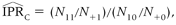
Our simulation results are shown in Figures 1 and 2 and Tables 1 and 2. We plotted the number of times each IPR estimate occurred during the 10 000 simulation trials. Each graph shows distributions of for three different exposure classification scenarios. For all experiments, the simulated expected value of was always within a few hundredths of the true value. We omit results for IPR_T = 1 in Tables 1 and 2 because in that case the null is true; hence there can be no bias towards the null, and both estimates always fall above (or below) the true null value ∼50% of the time.

Figure 1

Open in new tabDownload slide

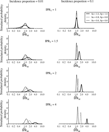
Distribution of , by IPR_T, incidence proportion in unexposed subjects, sensitivity and specificity where exposure prevalence = 0.5. , misclassified incidence-proportion ratio; IPR_T, true incidence-proportion ratio; Se, sensitivity; Sp, specificity; 10 000 simulation trials. Total number of exposed subjects = 5000, total number of unexposed subjects = 5000

Figure 2

Open in new tabDownload slide

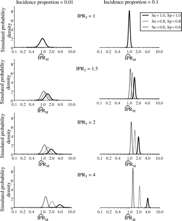
Distribution of , by IPR_T, incidence proportion in unexposed subjects, sensitivity and specificity where exposure prevalence = 0.1. , misclassified incidence-proportion ratio; IPR_T, true incidence-proportion ratio; Se, sensitivity; Sp, specificity; 10 000 simulation trials. Total number of exposed subjects = 1000, total number of unexposed subjects = 9000

As expected, bias was towards the null in all the situations we examined. That is, the expected value of was always between the null value of 1 and IPR_T for our simulation results (Tables 1 and 2). The magnitude of bias depended on sensitivity, specificity, exposure prevalence, and the true value. When the true IPRs were above 1, for a balanced population structure (i.e. P_E = 0.5) the exposure probability was above 0.5 among cases and hence the magnitude of bias was more influenced by sensitivity than specificity. However, when the exposure was uncommon (i.e. P_E = 0.1), the bias was more influenced by specificity.

Nonetheless, even though bias was towards the null and the process of exposure classification was non-differential, estimates could often be greater than the true value () (Figures 1 and 2, Tables 1 and 2). For example, when P_E = 0.5, IP₀ = 0.01, IPR_T = 1.5, and S₁ and S₀ = 0.80, in 19% of the simulation trials (Table 1). The proportion of times is indicated in Figures 1 and 2 as the area under the curves to the right of IPR_T. This proportion varied as a function of the true value, exposure prevalence, incidence proportion in the unexposed subjects, and sensitivity and specificity. It increased as the IPR_T decreased, P_E increased, IP₀ decreased, and S₁ and S₀ increased (Figures 1 and 2), situations in which the downward bias could easily be counterbalanced by upward random error. Larger sensitivity values had a greater influence on the proportion of times was greater than IPR_T for exposure prevalence P_E = 0.5, while specificity influenced this proportion more when exposure prevalence was 0.1.

Estimates were sometimes less than the null (). For example, when P_E = 0.5, IP₀ = 0.01, IPR_T = 1.5, and S₁ and S₀ = 0.8, in 9% of the simulation trials (Table 1). The proportion of times is indicated in Figures 1 and 2 as the area under the curves to the left of the null value. This proportion varied as a function of IPR_T, P_E, IP₀, and S₁ and S₀. It increased as the true value, exposure prevalence, incidence proportion in the unexposed subjects, and sensitivity and specificity all decreased (Figures 1 and 2), situations in which the downward random error could easily combine with downward bias to produce large downward total error.

Under some conditions, the misclassified estimates may lie almost entirely between the null and true value (), as illustrated by Figures 1 and 2. For example, when P_E = 0.1, IPR_T = 2, IP₀ = 0.1, and S₁ and S₀ = 0.80, all misclassified IPR estimates were between 1 and 2, that is the entire simulated distribution is between the null and true value (Figure 2). Thus, in some of the simulations, non-differential exposure misclassification did consistently lead to underestimation of the true value. This became more and more true as the true value increased, the baseline risk became larger, the exposure prevalence increased, and the misclassification probabilities became larger (Tables 1 and 2, Figures 1 and 2), situations in which the bias on the log scale would be nearer 50% and the random error would be small. This would also become more true as the sample size increased, for then the random error would decrease and bias would be the main determinant of the results.

Discussion

Because our simulation experiments satisfied the conditions for the non-differential misclassification rule, they all resulted in bias towards the null. With no misclassification (i.e. sensitivity and specificity = 1), a correctly classified estimate would exceed the true value in roughly half of the repetitions. When bias towards the null is added, it does become less probable that the estimate will exceed the true value, as long as any resulting increase in standard error does not exceed the bias. But it does not in general guarantee that the observed estimate will be an underestimate; in particular, non-differential exposure misclassification does not always result in an observed relative-risk estimate between the null and true value, even when it produces bias towards the null. Random error alone can cause an observed relative-risk estimate to be less than one or greater than the true value.

In summary, the belief that non-differential exposure misclassification always produces an underestimate of the true value is incorrect. One reason for this incorrect belief is a failure to understand that bias is not the only, or even necessarily, the main, source of error in an estimate. Bias is not the ratio of the observed estimate from one study to the true value, because the observed estimate also incorporates random errors. The latter errors diminish with sample size but remain substantial in most epidemiological studies, as revealed by the width of the confidence interval.

Another reason for the incorrect belief is the failure to recognize that non-differentiality is insufficient to guarantee the bias is towards the null; other conditions must be satisfied, especially independence of errors.^10,11,18,19 Furthermore, even small departures from non-differentiality can produce bias away from the null.¹² Finally, even when bias due to exposure misclassification is towards the null, other biases (such as confounding, selection bias, and mismeasurement of covariates) can cause the total bias to be away from the null. The combined effect from all biases must be considered when interpreting study results.^22–25

When biases are a serious concern (the usual case in epidemiology) and the study results are of potential policy importance, we recommend using quantitative methods for evaluating the effect of not only exposure misclassification but also other systematic errors.^19,22–30 Methods such as sensitivity analysis, uncertainty analysis, and bias modelling provide a means to account for systematic error in ways that do not depend on traditional and often faulty qualitative heuristics. These methods can be extended and given empirical grounding by the addition of ‘validation’ or reproducibility data to the analysis,^31,32 although very large amounts of such data may be needed to provide effective corrections,³³ and use of incorrect non-differentiality assumptions in the ensuing analyses may worsen bias.^34,35 When such methods are not used, we recommend that results be presented in a very cautious and descriptive manner, rather than promoted by unfounded judgments that biases are small or errors are in a known direction. We believe a very descriptive approach to presenting results is often commendable, and need not detract from the scientific value of a research report.³⁶

Simulation results such as ours are sensitive to the conditions chosen for the simulation. In practice one cannot show that a single epidemiological study has the conditions identical to those assumed in a simulation experiment. Thus, it may not be possible to generalize the details of our simulation results to many practical situations. They do not, for example, show how relaxing the strict non-differentiality or independence conditions would affect the behaviour of estimates. Nonetheless, they do show that even if the conditions are perfectly satisfied, the results may be an overestimate, with the probability of overestimation depending on the size of bias and the distribution of random errors. This point is important because any study is but one replication, and hence the results reflect random error as well as bias. Thus, unless the confidence intervals from the study are very narrow (suggesting random error is small), researchers should not infer that their results are an underestimate, even if they can persuasively argue that the net bias from all sources (not just exposure misclassification) is towards the null; the most that can be said is that the results are more likely an underestimate than an overestimate.

Disclaimer

Although the research described in the article has been funded in part by the US Environmental Protection Agency's STAR programme through grant (U-91615801-0), it has not been subject to any EPA review and therefore does not necessarily reflect the views of the Agency, and no official endorsement should be inferred.

This research has been supported by a grant from the US Environmental Protection Agency's Science to Achieve Results (STAR) programme.

References