
Causal mediation analysis in the context of clinical research
Introduction
In clinical research, a large number of variables may be collected and the relationship between each variable can be complex. The traditional method to explore the relationships between explanatory variables and outcomes is by using multivariable regression model. However, this method fails to disentangle mechanisms underlying the association between explanatory variable and outcome, while investigators are sometimes interested in such underlying mediating pathophysiological processes (1,2). In these situations, the investigators may have prior knowledge that an explanatory variable exerts its effect on outcome via direct and indirect pathways. In the indirect pathway, there is a mediator that transmits the causal effect. For example, suppose that corticosteroids are effective for reducing mortality rate of patients with acute respiratory distress syndrome (ARDS), and this effect is partly mediated by suppressing inflammatory response (3). In this scenario, corticosteroid treatment is an exposure, mortality is a binary outcome and inflammatory response is a mediator. It is interesting to explore how much of the total effect is transmitted via inflammatory response. The example motivates the causal mediation analysis (CMA). In this article, we will introduce a commonly used method for CMA proposed by Imai et al. (4). Its implementation with R package will be described in a step-by-step approach.
Understanding CMA
Suppose we have variables X and Y indicating the explanatory variable (or treatment variable) and outcome variable, respectively (Figure 1). Mediation in its simplest form is to add a mediator M between X and Y (5). Model-based mediation analysis is implemented in the mediation package (6). The sequential ignorability assumption should be satisfied for validity of the method used for this package. The assumption states that “the treatment (explanatory variable X) is first assumed to be ignorable given the pre-treatment covariates, and then the mediator variable (M) is assumed to be ignorable given the observed value of the treatment as well as the pre-treatment covariates.” (7). The first part is often satisfied by randomization while the second part implies that there are no unmeasured confounding between mediator and outcome, which is often questionable even in randomized trial. Moreover, this assumption is not verifiable in practice and sensitivity analysis should be performed to quantify the degree to which violation of the assumption would change the results. Sensitivity analysis will be described in detail in following sections. This section focuses on the model based mediation analysis with continuous outcome, which is based on three linear equations:

Y = i1 + cX + e1 [1]
Y = i2 + c'X + bM + e2 [2]
M = i3 + aX + e3 [3]
where i1, i2 and i3 denote intercepts, Y is the outcome variable, X is the explanatory variable, M is the mediator, c is coefficient linking X and Y (total causal effect), c' is the coefficient for the effect of X on Y adjusting for M (direct effect), b is the effect of M on Y adjusting for explanatory variable, a is the coefficient relating to the effect of X on M. e1, e2 and e3 are residuals (7) that are uncorrelated with the variables in the right hand side of the equation and are independent to each other. Under this specific model, the causal mediation effect (CME) is represented by the product coefficient of ab. Of note, Eq. [3] can be substituted into Eq. [2] to eliminate the term M:
Y = i2 + bi3 + (c' + ab)X + e2 + be3 [4]
It appears that the parameters related to direct (c') and indirect effect (ab) of X on Y is different from that of its total effect. That is, to testing the null hypothesis c=0 is unnecessary since CME can be nonzero even when the total causal effect is zero (i.e., direct and indirect effects can be opposite) (4,7), which reflects the effect cancellation from different pathways.
However, the above-mentioned equations within linear structural equation modeling (LSEM) framework are not directly applicable to binary outcome. LSEM equation needs extension to accommodate non-linear settings (8,9). In this article we will focus on Imai’s method that is applicable to non-linear settings (4).
Worked example
Next, a dataset is simulated using the motivating example described in the introduction section. Suppose investigators want to explore the effect of corticosteroids on mortality outcome, and it is valuable to notice if part of the total effect is mediated via reducing inflammatory response. C-reactive protein (CRP) is a biomarker of inflammatory response and there is evidence that higher CRP is associated with adverse clinical outcomes (10). Note that the example is created to demonstrate the use of CMA into the clinical context, and there is no clinical relevance of the results.

CMA
This article implements CMA using the R mediation package (6). This package also contains functions for CMA with certain designs or conditions such as multiple outcome/treatment/mediator combinations, multiple causal mechanisms, treatment non-compliance, and dataset with missing values. In addition, this package allows researchers to implement sensitivity analysis for certain parametric models. In the following example, the authors only applied the simplest form of CMA. Let’s first install the package and then perform CMA with a few lines of codes.

The mediate() function requires two fitted model objects: one is for the mediator and the other is for the outcome. In the example, the mediator model is a linear model that regresses crp on treat_flg. The outcome model is a logistic regression model that regresses mort on treat_flg and crp. Note that these two regression models allow other confounding factors to be added if they are observed. In the example, only the first 100 observations are used for analysis. The treat argument takes a character string indicating the name of the treatment variable (treat_flg) used in the models. Similarly, the mediator argument takes a character string indicating the name of the mediator variable (crp) used in the model.
Understanding summary output with binary outcome variable
The results of CMA can be accessed with summary() and plot() function.

The results show the ACME and average direct effect (ADE) for the treated and control groups. For a single index, researchers can use the average ACME and ADE to determine the average mediation strength. Note that the ACMEs are different for the treated and control groups. This can be understood in the counterfactual framework. Let’s first define ACME with mathematical equation according to Imai and colleagues (7):
δi(t) ≡ Yi [t, Mi(1)] − Yi [t, Mi(0)] [5]
δi(t) is the CME under treatment t, which represents the indirect effect of treatment on outcome Yi(t) through mediator. The subscript i indicates the individual patient. The counterfactual framework can be understood with the following question: what changes would occur to the outcome if the mediator is changed from the value under treatment t=1 [Mi(1)] to the value that would be observed under treatment t=0 [Mi(0)], while holding treatment at t. While the outcome of the form Yi[t, Mi(t)] is observable, Yi[t, Mi(1−t)] is unobservable for a given patient. In the example, CME (treated, δi(1)) is the difference between two potential mortality outcomes for patient i who received corticosteroids. For the patient, Yi[1, Mi(1)] is observed outcome if he or she receives corticosteroids, whereas Yi[1, Mi(0)] represents the mortality outcome under the condition that the patient still receives corticosteroids but change the mediator value that would result without treatment. This definition with counterfactual framework reflects the intuitive notion of mediation that the treatment indirectly influences outcome via mediator. Similarly, direct effect can be defined as:
ζi(t) ≡ Yi [1, Mi(t)] − Yi [0, Mi(t)] [6]
In the example, ζi(1)represents the direct effect of corticosteroids on patient i’s mortality outcome while holding the crp at the level that would be observed under treatment. The causal effect of the treatment on the outcome for unit i now can be defined as the following relationship
Total ≡ δi(t) − ζi(1−t) [7]
While CME is at the individual level, the ACME is the expected value for the whole study population:

It appears that ACMEs of both the treated and the control are statistically non-significant. This may be due to the limited sample size. Recall that we only used the first 100 patients for analysis. The results can be visualized with plot() function.

The simple function automatically produces a plot of mediation analysis. Estimates for both treated and control group were depicted because they are different in the example. The dashed line represents the control and solid line represents the treated. It appears that most of the total effect is explained by the direct effect (Figure 2).

The next question that often confuses people is the interpretation of coefficients. In normal linear model, all variables are linked in the same scale and the interpretation is straightforward. However, in CMA with binary outcome variables, the estimated coefficients from above links to the probability scale, rather than that obtained from logistic regression model that its exponentiation gives the odds ratio (OR). Next, let’s take a look at how estimation of mediation effects can be different using different methods: the standard LSEM approach proposed by Baron (11) and the method by Imai.
Imai’s method consists of two steps which are based on Eqs. [5] and [6]. The first step is to fit regression models for mediator and outcome, which has been done in the above R codes. The second is to simulate the unobserved potential mediator and then compute the average potential outcome from the fitted model.

The value 0.193 approximate the ACME(0) reported in tabular output by summary() function. A small diffidence is that we perform limited number of simulations. If we compute acme0 with our code 1,000 times and take the average, the value would be more approximate. The coefficients estimated with mediate() function can be better understood with above explicit computation. Because the type argument takes a string variable “response” within the predict() function, y0_m0 is the probability of death for a given patient in the control group and a crp level being observed. y0_m1 is the probability of death for a given patient in the control group and a crp level that would be observed supposing the patient had received treatment. Thus, y0_m1 is unobservable in reality but only in counterfactual framework. The difference between y0_m0 and y0_m1 gives the ACME in the control group that can be interpreted as the probability of death being changed by varying crp values, while holding the treatment status constant. The total effect of 0.94 can be interpreted as the increased probability of death comparing treatment versus control group. The model coefficients estimated from Imai’s nonparametric method have a direct link to the probability scale and thus is more clinically relevant.
Now we will show that if we ignore the fact that some of the equations are fit with nonlinear link and still use the formula derived from linear setting, i.e., the total effect c = c’+a*b, we will not be able to yield correct result. Eqs. [2] with logit link and [3] have been fitted and stored in objects model.y and model.m, respectively. We only have to fit the Eq. [1] with logit link and store it in an object called model.t.

The results show that the total effect estimated from regression model.t approximate that estimated from regression models.y and model.m. For nonlinear case, the two quantities might approximately the same under some special cases, for example, weak indirect effect (a*b), log link function or rare outcome. Our example is the one with weak indirect effect. However, the values of these estimated coefficients are not equal to that obtained via mediate() function, because the later coefficients are identified with methods as described above (12). The coefficients estimated from logistic regression model are in the linear prediction function scale that its exponentiation gives the odd ratio (OR).

The total OR is the sum of direct effect OR and indirect effect OR. The results show that there is negligible indirect effect, and the direct effect takes nearly all of the total effect.
Sensitivity analysis
CMA described above is performed under sequential ignorability assumption. However, this assumption is untestable in practice. One approach is to perform sensitivity analysis to examine whether the results are robust to the violation of the assumption. Violation to assumption indicates that there exists an unmeasured confounder that is related to both the mediator and the outcome. Note that this unmeasured confounder is not affected by the treatment. Sensitivity analysis uses certain statistics to quantify how strong the confounder would have to be to change the conclusion being drawn about the direct and indirect effect (13). Imai and colleagues proposed a correlation parameter (ρ) reflecting the existence of omitted variables that were related to the mediator and outcome even after conditioning on treatment, and the parameter was added to the calculations of ACME. Sensitivity analysis is to vary ρ values and compute corresponding ACMEs. There are two methods to calculating ρ. One is to compute ρ based on residual correlation:
ρ ≡ cor(e2, e3) [9]
The other way is to calculate correlation parameter ρ based on coefficients of determination (i.e., a number that indicates the proportion of the variance in the dependent variable that is predictable from the independent variable):
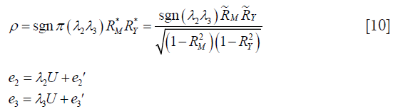
Where  and
and  represent the proportion of previously unexplained variance (mediator and outcome) that is explained by the unobserved confounders.
  and
and  are the proportion of variance that is explained by the unobserved confounders. U is unobserved confounding variable.
  and
and  are the coefficients of determination for the mediation and outcome regression models. represents the proportion of explained variance by covariates in the mediation model (Eq. [3]). λ2 and λ3 are coefficients for unobserved variable in the equation regressing residual e2 or e3 on the unobserved variable. We only care about the direction (sign) of the effect. In this framework, investigators can specify values of (, ) and (, ), and the sign of (λ2λ3) to estimate ACME (4,14).
Next I proceed to perform sensitivity analysis with medsens() function. Because the function in its current version only support probit link, the mediation model needs to be updated.

The medsens() function first takes an object of class “mediate” which is an output object from mediate() function. The argument rho.by takes a numeric value ranging from 0 to 1 indicating the increment for sensitivity parameter ρ. The effect.type argument indicates which effect to be examined.

Because we assigned “indirect” for the argument effect.type, sensitivity analysis for ACME is performed. The summary output displays the computed ACMEs by varying ρ values for the treatment and control groups. Two tables are similar in interpretation, so we only take a look at the first table (control group). The first column is the ρ values with an increment of 0.1. The second column shows the corresponding ACMEs, and the third and forth columns are confidence intervals. The last two columns are quantities based on coefficients of determination. Because the ρ value at which ACME becomes zero is of interest, it is displayed following the table. A graphical display of the results can be more intuitive and helpful in sensitivity analysis.

The sens.par argument specifies which sensitivity parameter, residual correlation or coefficients of determination, to be displayed. The dashed line represents the ACME value without correlation (ρ=0), which is computed under the assumption of sequential ignorability. We need to set ρ≥0.3 for the ACME to become negative (Figure 3). A large critical ρ value is needed to reverse the sign of ACME indicates the robustness of the result to the violation of ignorability assumption. It requires subject knowledge to judge whether the value of 0.3 is large or not. In practice, observed confounding variables are often used to determine the upper bound of sensitivity parameters.

Sensitivity analysis based on R2 statistic is performed by assign “R2” to sens.par. The type of R2 to be used is specified in r.type argument. A string variable “residual” indicates that the effects are plotted against the proportions of the residual variances that are explained by the unobserved confounder. On the other hand, a value of “total” indicates that the proportions of the total variances are used as sensitivity parameters. When sensitivity analysis is performed with R2 statistic, the user must specify whether the unobserved confounder affects the mediator (λ3) and outcome (λ2) in the same direction (sgn[λ2λ3]=1) or opposite direction (sgn[λ2λ3]=−1). If the effects are in the same direction, users assign sign.prod = “positive”. Otherwise, the sign.prod argument takes the string variable “negative”.

Four plots are produced by varying r.type and sign.prod arguments (Figure 4). The first panel shows the sensitivity analysis for ACME in the control group by setting sgn(λ2λ3)=−1. However, it appears that except for the first plot that displayed many values of ACME, each of the other plots only displays the contour of one ACME value. The reason is that the native R contour function automatically adjusts the displaying values, and thus we need to adjust the levels argument to allow displaying of more contours. The ACME values across a range of degrees of confounding can be examined in the values returned by the medsens() function.


Note that the ACME values (i.e., the first 9 values of the sens.out$d0 output) for the control group when sgn(λ2λ3)=−1 is increased at a step approximating 0.1 and thus can be displayed without specifying levels argument. However, the ACME values (i.e., the first 9 values of the sens.out$d1 output) for the treated group when sgn(λ2λ3)=−1 is changed at steps significantly different from 0.1, thus we need to specify the levels for displaying more contours.

The bold line represents various combinations of R2 statistics where ACME takes the value zero (Figure 5). In the example, the value of ACME under sequential ignorability assumption is not statistically significant, thus the degree of confounding where ACME would be zero is of limited interest. In other situations, where ACME is statistically significant, the critical point of the degree of confounding where ACME takes zero is of great interest because beyond this point the effect size is in opposite direction (i.e., the sign is changed). However, there is no cutoff value for the statistics of confounding (i.e., ρ and combinations of R2 statistics) to judge the robustness of CMA results estimated under ignorability assumption.

Acknowledgements
None.
Footnote
Conflicts of Interest: The authors have no conflicts of interest to declare.
References
- MacKinnon DP, Pirlott AG. Statistical approaches for enhancing causal interpretation of the M to Y relation in mediation analysis. Pers Soc Psychol Rev 2015;19:30-43. [Crossref] [PubMed]
- Linden A, Karlson KB. Using mediation analysis to identify causal mechanisms in disease management interventions. Health Serv Outcomes Res Method 2013;13:86-108. [Crossref]
- Zhang Z, Chen L, Ni H. The effectiveness of Corticosteroids on mortality in patients with acute respiratory distress syndrome or acute lung injury: a secondary analysis. Sci Rep 2015;5:17654. [Crossref] [PubMed]
- Imai K, Keele L, Tingley D. A general approach to causal mediation analysis. Psychol Methods 2010;15:309-34. [Crossref] [PubMed]
- MacKinnon DP, Fairchild AJ, Fritz MS. Mediation analysis. Annu Rev Psychol 2007;58:593-614. [Crossref] [PubMed]
- Tingley D., Yamamoto T, Hirose K, et al. mediation: R Package for Causal Mediation Analysis. J Stat Softw 2014;59:1-38. [Crossref] [PubMed]
- Imai K, Keele L, Yamamoto T. Identification, Inference and Sensitivity Analysis for Causal Mediation Effects. Statistical Science 2010;25:51-71. [Crossref]
- Li Y, Schneider JA, Bennett DA. Estimation of the mediation effect with a binary mediator. Stat Med 2007;26:3398-414. [Crossref] [PubMed]
- MacKinnon DP, Lockwood CM, Brown CH, et al. The intermediate endpoint effect in logistic and probit regression. Clin Trials 2007;4:499-513. [Crossref] [PubMed]
- Zhang Z, Ni H. C-reactive protein as a predictor of mortality in critically ill patients: a meta-analysis and systematic review. Anaesth Intensive Care 2011;39:854-61. [PubMed]
- Baron RM, Kenny DA. The moderator-mediator variable distinction in social psychological research: conceptual, strategic, and statistical considerations. J Pers Soc Psychol 1986;51:1173-82. [Crossref] [PubMed]
- Imai K, Keele L, Tingley D, et al. Unpacking the Black Box of Causality: Learning about Causal Mechanisms from Experimental and Observational Studies. American Political Science Review 2011;105:765-89. [Crossref]
- VanderWeele TJ. Mediation Analysis: A Practitioner's Guide. Annu Rev Public Health 2016;37:17-32. [Crossref] [PubMed]
- Imbens GW. Sensitivity to Exogeneity Assumptions in Program Evaluation. American Economic Review 2003;93:126-32. [Crossref]

