
A Comparison of Partial Volume Correction Techniques for Measuring Change in Serial Amyloid PET SUVR
Abstract
Longitudinal PET studies in aging and Alzheimer’s disease populations rely on accurate and precise measurements of change over time from serial PET scans. Various methods for partial volume correction (PVC) are commonly applied to such studies, but existing comparisons and validations of these PVC methods have focused on cross-sectional measurements. Rate of change measurements inherently have smaller magnitudes than cross-sectional measurements, so levels of noise amplification due to PVC must be smaller, and it is necessary to re-evaluate methods in this context. Here we compare the relative precision in longitudinal measurements from serial amyloid PET scans when using geometric transfer matrix (GTM) PVC versus the traditional two-compartment (Meltzer-style), three-compartment (Müller-Gärtner-style), and no-PVC approaches. We used two independent implementations of standardized uptake value ratio (SUVR) measurement and PVC (one in-house pipeline based on SPM12 and ANTs, and one using FreeSurfer 6.0). For each approach, we also tested longitudinal-specific variants. Overall, we found that measurements using GTM PVC had significantly worse relative precision (unexplained within-subject variability ≈4–8%) than those using two-compartment, three-compartment, or no PVC (≈2–4%). Longitudinally-stabilized approaches did not improve these properties. This data suggests that GTM PVC methods may be less suitable than traditional approaches when measuring within-person change over time in longitudinal amyloid PET.
INTRODUCTION
Positron emission tomography (PET) scans typically have an effective spatial resolution of approximately 6–10 mm but are reconstructed into much smaller voxels. As a result of this in combination with other technical factors (e.g., scatter, randoms, etc.), many PET image voxels contain partial volume effects: the signal within a voxel is effectively an average of signals from several neighboring types of tissue and/or brain/non-brain regions after convolution with a point spread function (PSF) that is much larger than the voxel size. Many techniques have been proposed for partial volume correction (PVC) of PET images, which typically leverage corresponding higher-resolution images, such as structural magnetic resonance imaging (MRI), to estimate the sources of these combined voxel measurements and generate corrected measurements and images. Many publications have reviewed and compared these techniques [1–9]. Among studies measuring proteinopathies associated with Alzheimer’s disease (AD), however, a consensus has not been reached for which, if any, PVC method should be applied.
Inherently, PVC amplifies measurement noise in trying to reduce measurement bias, because numeric measurements in voxels with lower signal are boosted to compensate for lesser amounts of tissue available for potential tracer binding. Existing validations and comparisons of PVC methods have examined the effects of various PVC methods using phantoms, simulations, and group-wise discrimination in cross-sectional patient-group comparisons [4, 8, 10–14]. Clinical trials and observational cohort studies of aging and AD rely on measurements of change over time (i.e., slope) from serial PET images. Over a typical 1–3 year study period, rates of change tend to be small, and group-wise differences in rates of changes are typically smaller than those in cross-sectional measurements, which measure accumulated total pathology throughout the lifespan [15]. Therefore, it is necessary to re-evaluate whether each method is appropriate for this context.
In this work, we compare several popular PVC approaches: no PVC, two-compartment [16], three-compartment [12], and geometric transfer matrix (GTM) [13], specifically for the task of measuring change over time by using a large cohort of subjects each with three timepoints of Pittsburgh Compound B (PiB) amyloid PET [17]. To confirm that our findings are inherent to the PVC algorithms used and not to specific implementations, we evaluate two independent measurement pipelines and implementations of each major PVC approach.
MATERIALS AND METHODS
Subject characteristics
We perform our comparisons using existing scans of subjects (n = 278) selected from the Mayo Clinic Study of Aging (MCSA) and Mayo Alzheimer’s Disease Research Center (ADRC) studies. MCSA is a longitudinal cohort study of cognitive aging based on a random sample of Olmsted County, Minnesota residents [18, 19]. The ADRC study recruits and follows subjects initially seen as patients at the Mayo Clinic Neurology practice. Subjects were required to have three 3T MRI and PiB PET scans over approximately 3.5 years. We required three timepoints because this allows a more accurate assessment of between-subject versus within-subject variability. All studies were approved by their respective institutional review boards and all subjects or their surrogates provided informed consent compliant with HIPAA regulations. We provide a table of demographics in Table 1.
Table 1
Subject Demographics
| Characteristic | Summary |
| Number of subjects | 278 |
| Sex, n (%) | |
| Female | 108 (39%) |
| Male | 170 (61%) |
| Age at baseline PET, y | 75 (70, 79) [51, 93] |
| Education, years | 15 (12, 17) [0, 24] |
| Global cortical PIB, SUVR | 1.39 (1.31, 2.02) [1.13, 3.20] |
| Diagnosis at baseline, n (%) | |
| CU | 179 (64%) |
| MCI | 62 (22%) |
| Dementia | 37 (13%) |
| APOE ɛ4, n (%) | |
| Carrier | 102 (37%) |
| Non-carrier | 176 (63%) |
| MMSE score | 28 (27, 29) [8, 30] |
| Time between first and | 3.7 (2.5, 4.1) [1.6, 5.7] |
| third scan, y | |
| Time between corresponding | 7 (1, 20) [0, 148] |
| MRI and PET scans, daysa |
Values are given as: median (1st quartile, 3rd quartile) [min to max] or number (percent) n, number of subjects; CU, clinically unimpaired; MCI, mild cognitive impairment; APOE, apolipoprotein E; MMSE, Mini-Mental State Examination. aBased on all scans for all individuals.
Scan parameters
T1-weighted MRI scans (used for atlas normalization/masking, and for PVC where applicable) were acquired using 3T scanners manufactured by General Electric (GE) (models Discovery MR750, Signa HDx, Signa HDxt, and Signa Excite) using a 3D Sagittal Magnetization Prepared Rapid Acquisition Gradient-Recalled Echo (MP-RAGE) sequence. Repetition time (TR) was ≈2300 ms, echo time (TE) ≈3 ms, and inversion time (TI) = 900 ms. Voxel dimensions were ≈1.20 mm×1.015 mm×1.015 mm. All images were acquired using 8 channel head array receiver coils.
PiB PET scans were acquired using GE scanners (models Discovery 690XT and Discovery RX; GE Healthcare, Waukesha, WI). Subjects were injected with PiB (628 MBq; range 385–723 MBq) and a low dose CT scan was acquired for attenuation correction. Beginning 40 min post-injection, subjects then underwent a 20 min dynamic PET scan with four 5 min frames. Dynamic PET images were generated (256 matrix, 300 mm field of view, 1.17 mm×1.17 mm× 3.27 mm voxel size) using fully-3D [20] or Fourier-rebinned [21] OSEM iterative reconstruction algorithms with 3 iterations and 35 subsets. Standard corrections for attenuation, scatter, random coincidences and decay were applied as well as a 5 mm Gaussian post-reconstruction filter. The four-frame sequences were inspected by technicians for excessive motion, which was not found in any of the included scans. The images from the four dynamic frames were averaged to create a single static image.
Partial volume correction methods
No PVC
Although partial volume correction of PET images was first proposed decades ago [11, 22] and the methodology has continued to flourish, no strong consensus has emerged for which method is best, and publications using data without partial volume correction are still frequent in the literature. We include no-PVC as an option in this comparison to provide a reference measurement of how much variance is present in serial amyloid PET standardized uptake value ratio (SUVR) measurements without PVC, in the context of serial measurements.
Two-compartment (Meltzer-Style) PVC
Two-compartment (Meltzer-style) PVC is a voxel-based approach where each voxel is modeled as a linear combination of only two classes: tissue and non-tissue. This is one of oldest and most common methods for PVC, in part because it is easy to understand and implement. PET is coregistered to the corresponding MRI and the MRI is segmented to mark each voxel as either tissue or non-tissue. A mask of voxels segmented as tissue is then blurred by the assumed scanner PSF to produce an estimate of the fraction of tissue-originated signal contained in each PET image voxel. Individual PET scan voxels are then each divided by this estimated tissue fraction to correct for partial volume. The signal in non-brain voxels is, implicitly, assumed to be zero. For example, if a PET voxel is estimated to contain 80% tissue and 20% non-tissue according to the PSF-blurred MRI segmentation, its raw intensity is divided by 0.8 to estimate what the signal may have been if the voxel contained 100% tissue [16].
Three-compartment (Müller-Gärtner-style) PVC
Three-compartment PVC is also a voxel-based method that extends the two-compartment model such that uptake in gray matter and uptake in white matter (WM) are modelled separately, rather than together as a single “tissue” class. PET is coregistered to the corresponding MRI and the MRI is segmented to mark each voxel as gray matter, WM, or non-tissue. An atlas is used to locate and measure the mean PET signal inside the centrum semiovale, a large central region of WM. It is assumed that all WM has homogeneous uptake equal to this value, which is then assumed to be the partial volume corrected value for WM (we also examine a less-common, alternative method of estimating WM signal in the Supplementary Material). A binary mask of voxels segmented as WM is blurred by the PSF to produce an estimate of the fraction of WM-originated signal in each PET image voxel. This is then multiplied by the value from the centrum semiovale to estimate the contribution of WM to measured signal in each voxel. The resulting WM-contribution image is subtracted from the original PET image to remove WM signal in each voxel. Finally, the steps from two-compartment PVC (above) are performed on the resultant image to also correct for the effects of non-tissue voxels [12].
Geometric transfer matrix (Rousset-Style) PVC
GTM PVC, also known as region spread function (RSF) PVC, is a region-based method proposed by Rousset et. al. in 1998. Brain PET images are parcellated into many individual regions using MRI segmentation and atlas propagation, and the method attempts to model PSF interactions between entire regions (rather than voxels individually, as in two- and three- compartment PVC). PET signal values within each region are modelled as homogeneous. Consider n regions of interest. Each region (i) is individually segmented and convolved with a 3D Gaussian kernel with the width of the estimated PET PSF. This creates a probabilistic map, called a regional spread function (RSFi), of how much signal from region i is assumed to be present in each image voxel. The mean RSF value is calculated within each original region of interest (j) to compute an estimate of signal from region i appearing in region j. The GTM model assumes that the observed PET signal in each region is the sum of true (unknown) PET signals in each region combined in a weighted sum where the mean RSF values serve as the weights. This leads to a system of linear equations which may be solved for the unknown, ideal (as if there were no PSF) regional PET values. For an atlas with n ROIs, each of these n equations with n unknowns is inserted into a n×n matrix of equations. Standard matrix methods are then used to solve for the n unknown, PVC-corrected values [13].
Unlike the voxel-based methods, GTM PVC attempts to correct for the effects of PSF causing wash-in and wash-out of signal between neighboring regions, rather than only between broad classes of tissue and non-tissue. A modification of GTM called Symmetric GTM has also been proposed, where the initial uncorrected per-ROI values are measured from the PSF-blurred ROIs (RSFs), rather than the un-blurred binary masks, to improve bias and noise characteristics [23]. This symmetric variant was recently included as the recommended PET PVC method in the latest 6.0 release of the popular FreeSurfer package [24], facilitating its proliferation.
SUVR measurement pipelines
Our goal in this work is to examine properties intrinsic to the PVC methods themselves, rather than specific implementations. To this end, we compared two sets of wholly-independent software pipelines using the same input scans.
Mayo SUVR pipelines
In this work we refer to a set of in-house software for calculating SUVR values from pairs of MRI and PET images as the Mayo SUVR pipelines. These are based primarily on components from the Statistical Parametric Mapping version 12 (SPM12) [25] and Advanced Normalization Tools (ANTs) [26] packages, and templates/atlases from our own Mayo Clinic Adult Lifespan Template (MCALT) package [27] (https://www.nitrc.org/projects/mcalt/). We have used these components to implement two pipeline variants: a cross-sectional variant where values for each timepoint are computed using only images from that timepoint, and a longitudinal variant where values for each timepoint are computed using images from all timepoints simultaneously. We describe both in this section.
Preprocessing
All input images were converted to nifti format from DICOM. MRI were additionally corrected for through-plane gradient distortion [28] (correction in the sagittal plane was performed on the scanner). These preprocessed images were directly used as inputs for both the Mayo and FreeSurfer pipelines described below.
Cross-sectional variant.
The cross-sectional Mayo PiB SUVR pipeline has been previously described [15, 29]. More recently we have updated it to use the MRI segmentation/normalization steps previously described in [30], and we use this version here. In brief, PET scans were normalized to the corresponding MRI using a 6DOF (rigid) transform computed with SPM12 and resampled using B-spline interpolation. We chose B-spline, rather than linear interpolation, to minimize unnecessary loss in image clarity due to resampling. Although a full comparison of PET image resampling methods is beyond the scope of this paper, we also replicated all of our experiments using linear interpolation and found no significant quantitative differences in measurement reproducibility for any variants (data not presented). The corresponding MRI was corrected for intensity inhomogeneity and segmented with Unified Segmentation [31] in SPM12 using MCALT tissue priors and segmentation parameters. Normalization parameters were calculated between the intensity-corrected MRI and the MCALT T1-weighted template using ANTS symmetric normalization [32], and MCALT atlases were transferred to the MRI space using ANTs’s GenericLabel interpolation. Atlas regions were masked to only include voxels of their corresponding tissue type(s) according to the MRI segmentation, and mean values within each region were computed. The “GlobalPiB” target region is a composite that includes the prefrontal, orbitofrontal, parietal, temporal, anterior cingulate, and posterior cingulate/precuneus regions [29]. A mask of this composite is available in the public MCALT release. Since the best way to normalize PET uptake is still an active area of research, we compared methods across a number of reference regions. The cerebellar crus, cerebellar gray matter, whole cerebellum, and pons reference regions were each defined using MCALT atlases. The supratentorial WM reference region was defined by using the MCALT lobar atlas to remove cerebellar/brainstem regions from a mask of voxels segmented as WM according to the MRI. Eroded supratentorial WM reference regions have been proven effective for serial amyloid PET analysis [33–36], but we included this region without erosion because FreeSurfer/PETSurfer contains no straightforward mechanism to erode WM regions or otherwise separate subcortical from deep WM regions. We do not advocate using non-eroded WM reference regions for amyloid PET due to contamination from gray matter signal, but we included this region in our comparisons because this was the only supratentorial WM region that we could implement similarly with both pipelines. A flowchart of the overall Mayo cross-sectional pipeline is available in Supplementary Figure 2.
Longitudinal variant.
The Mayo longitudinal PET processing pipeline uses the same key components as the cross-sectional pipeline, but critically differs such that all steps are performed by simultaneously using data from all available timepoints in an attempt to stabilize the resulting registrations, segmentations, and parcellations [37]. This approach creates a single-subject template (SST) for each subject’s set of serial PET images (PET-SST), and one for each subject’s set of MRI scans (MRI-SST).
Each MRI-SST was formed by using the buildTemplateParallel iterative group-wise nonlinear registration approach from ANTs [38] to build a mean-space template of all the MRI timepoints. This single image was then segmented and parcellated into regions using the same methods (SPM12, ANTs, MCALT) as in our cross-sectional approach described above, and used for quantifying each PET scan in place of that timepoint’s original MRI. We chose to segment the mean-timepoint image directly and use it for all timepoints, rather than segmenting each timepoint after resampling it to this mean space. We made this choice because conceptually it favors stability (only a single consistent segmentation/parcellation) over accuracy (tissue boundaries in the mean-space image less accurately match any of the individual timepoints). This is more distinct from the cross-sectional approaches and from the Longitudinal FreeSurfer approach, which we also compare. Thus, this choice compares a wider diversity of approaches. During a preliminary phase of this study, we compared a variant with individual-timepoint segmentations/parcellations in the mean space, and the results were not significantly different from the presented variant. For longitudinal studies with a longer time span, where intra-subject differences in atrophy would be larger, we would expect the differences between these approaches to be larger and the re-segmentation approach would be more appropriate. Approaches using similar principles have been shown to improve the reliability and biological plausibility of change measurements using MRI [39].
PET scans from all time points were coregistered to a common space to create a PET-SST using an in-house groupwise registration based on 6-DOF spm_coreg. First, each timepoint was independently 6-DOF-registered to the MCALT_T1 template and resampled in this space. A voxel-wise mean was calculated, forming an initial PET-SST. Each PET scan was then registered to this initial PET-SST, then a new mean was calculated, and the process was repeated for a total of 3 times to form the final PET-SST. A single rigid registration between the MRI-SST and PET-SST was calculated, and each PET scan was resampled (B-spline) to the space of the T1-SST by a composite of the PET⟶PET-SST transform and the PET-SST⟶T1-SST transform. Each of these transformed PET scans was then used with the segmentations/parcellations of the MRI-SST for SUVR quantification and PVC.
To summarize this process, all PET timepoints for a subject were quantified using a single, mean-space MRI of that subject that was derived from all its MRI timepoints. This approach of using a single mean-space MRI for all PET timepoints is designed to minimize variation due to instabilities across timepoints in the MRI processing steps (intensity inhomogeneity correction, segmentation, and atlas registration/parcellations). A mean-space single-subject PET template was also formed, and a single rigid transform was used between the PET and MRI modalities by computing a registration between both templates. This approach of a single PET-MRI registration is designed to minimize the effects of PET-MRI registration instability, which we have previously documented [40]. All steps were performed such that all timepoints were treated equally, to avoid causing bias [41] as in approaches that, e.g., resample all timepoints to match the baseline. We provide a flowchart of all steps in this method in Supplementary Figure 2.
2-compartment and 3-compartment PVC implementations.
For the Mayo pipelines we used in-house implementations of 2- and 3-compartment PVC according to the methods in the original studies [11, 12]. We applied these voxel-based corrections directly prior to calculating the mean values in each atlas region. We used tissue segmentations of the subject MRI from SPM12 as described above, and assumed a PSF of 8 mm full width at half maximum (FWHM). This value was determined by averaging transaxial and axial PSF measurements from an internal study of scans using a F-18 point source at the center of a water phantom, reconstructed identically to the brain imaging protocols.
GTM PVC implementation.
For the Mayo pipelines, we adapted the core GTM PVC logic from a publically-available Matlab implementation of Rousset-style GTM PVC [42]. That implementation was specifically designed for tau PET and to use FreeSurfer brain parcellations as inputs, but it is completely distinct from the PETSurfer implementation later included in FreeSurfer 6.0. Our in-house adaptations only retained the core Rousset-style GTM PVC logic (i.e., RSF estimation and matrix solving) from this implementation. We rewrote the functions around this core to instead use input regions from a combination of our SPM12 MRI segmentations and MCALT atlas regions (instead of FreeSurfer segmentations) to create a dense 132-region atlas where every voxel is included, analogous to but distinct from the gtmseg step in PETSurfer (below). To form these regions, structures in the MCALT_122 and MCALT_Lobar atlases were first parcellated as such, and then classes for cerebrospinal fluid, air, skull+dura, and WM were added using the SPM12 segmentations. We did not include regions/corrections for extra-cortical hotspots from the Baker implementation, because these are specific to tau PET. Unlike FreeSurfer, our atlas splits WM into subcortical and deep WM, but to match FreeSurfer’s regions we combined these afterward to form a total supratentorial WM reference region. As with the voxel-based methods, we assumed a PSF of 8 mm FWHM.
PETSurfer (FreeSurfer 6.0) SUVR pipelines
FreeSurfer is a widely-used software package for surface-based analysis of brain MRI [43]. FreeSurfer analyses can be performed using either the cross-sectional stream or the longitudinal stream, which segments all serial timepoints at once for increased longitudinal stability [44]. In version 6.0, FreeSurfer introduced a new module called PETSurfer, which is used to register a PET scan to a corresponding, previously-segmented MRI and output tables of PET values in each atlas region [45]. Regional values can be output either with or without GTM PVC applied. PETSurfer has no longitudinal pipeline for analyzing serial PET scans using multiple timepoints simultaneously; however, when analyzing PET scans it can use MRI segmentations that were produced using either the cross-sectional or the longitudinal FreeSurfer pipeline, and the latter serves as the recommended approach for serial data [46].
We first preprocessed MRI scans by converting to nifti format and correcting for gradient unwarping as in the Mayo pipelines described above. After this preprocessing, we used PETSurfer with FreeSurfer 6.0 to produce uncorrected and symmetric-GTM-corrected ROI values using standard settings and PETSurfer procedures (https://surfer.nmr.mgh.harvard.edu/fswiki/PetSurfer). We refer to values produced using the cross-sectional MRI segmentations as FreeSurfer_CrossSec, and those using the longitudinal segmentations as FreeSurfer_Longitudinal. As in the Mayo pipelines, we assumed a PSF of 8 mm FWHM. For each reference tested reference region, we used the –rescale option to mri_gtmpvc to provide the appropriate region number(s). To form a composite target region from FreeSurfer’s atlases that is analogous to our GlobalPiB composite region, we used a size-weighted mean of PETSurfer’s output regional SUVR values (with each choice of reference region) of all cortical regions except for those marked as occipital, pre/postcentral, and insula.
Statistical methods
In this section, we detail the statistical methods by which we comparatively evaluate SUVR pipelines. All statistical analyses were performed using R version 3.3.1 (https://www.r-project.org/).
Data inspection and preprocessing
We first performed a graphical analysis of outliers and noticed the presence of a small fraction of extreme values due to failures in segmentation or registration. Based on this preliminary analysis, we chose to treat SUVR values that were outside the range of [0,7] as pipeline failures. Although amyloid PET SUVR values of up to 6 would be extremely large by standard SUVR measures, such values are not uncommon when using GTM PVC, and we wanted to use a standard threshold for all methods. Using these thresholds, we identified any subjects for which any method produced an SUVR value that was either outside this range, or not a number (i.e., zero-mean or zero-voxel reference regions). This occurred for only two subjects (1 clinically unimpaired (CU), 1 mild cognitive impairment (MCI)), which we excluded from all further analyses. Next, we identified n = 11 subjects (8 CU, 1 AD, 1 other) that did not have exactly three timepoints of computed SUVR values with every method due to failures in imaging processing pipelines. All of these were failures from FreeSurfer-based methods (no failures were observed with the Mayo methods). Further analyses continued with the remaining n = 278 subjects.
SUVR values from the FreeSurfer pipeline were then plotted versus those from the Mayo pipelines separately by reference region and PVC method in order to validate each of these independent implementations by examining to what extent the estimates agreed (i.e., clustered about the identity line, y = x) and their correlation (i.e., clustered about a regression line).
Estimating the coefficient of variation for each method
We used linear mixed effects regression to model natural logarithm transformed SUVR values over time to estimate the magnitude of within-subject variation for a given measurement method. Even in relatively homogeneous populations PET SUVR values tend to be right skewed due to measurement errors being proportional rather than additive. After a log transformation, SUVR values tend to be approximately normally distributed and have variance that is comparable across the log(SURV) distribution and therefore approximately additive. By a property of the log-normal distribution, the standard deviation (SD) of log-transformed values equals the coefficient of variation (CV) of the original distribution, where CV is the SD divided by the mean. We therefore interpret the residual standard deviation from a mixed of log-transformed SUVR values as providing an estimate of the CV of the method and an indication of the magnitude of within-subject measurement error.
For our primary analysis, our mixed model specification was as follows: We treated time from baseline as a fixed effect and included a random intercept and a correlated random slope for each individual. For each individual, time zero was defined as the midpoint between the first and third scan. We used the arm package’s sim() function [47] to perform 10,000 parametric bootstrap/posterior simulations of the mixed-effects model regression coefficients and variance parameters for each method. We used these simulations when plotting means and 95% confidence intervals.
We assume that change in SUVR over relatively short intervals can be modelled as linear and that deviations from linearity can primarily be attributed to measurement error that an ideal method would minimize. However, fitting a least squares line for each subject results in a high degree of overfitting and would severely underestimate the residual error. By using a mixed model approach, individual intercepts and slopes are shrunk toward the overall population average to reduce overfitting and account for regression to the mean. The resulting model-based residual SD arguably better reflects the true CV of the measurements.
Our justifications for these assumptions have been previously published [36]. In brief, we wish to penalize methods that produce biologically implausible triangle-shaped trajectories (i.e., where values strongly increase and then decrease, or vice versa, over short intervals of time). It is known that amyloid PET trajectories in AD subjects are a roughly sigmoidal shape [15] with an accumulation period of ≈19 years [48]. Having three measurements over a span of ≈3 years, it is reasonable to assume that trajectories should be locally linear. Therefore, we consider significant acceleration or deceleration in measured SUVRs to be much more likely due to measurement error than a true change in amyloid.
Group-wise differences in slopes
To assess how each method might perform for a hypothetical study comparing rates of amyloid accumulation across two groups, we performed a second statistical analysis wherein we separated our subjects into two groups: clinically unimpaired and clinically impaired (MCI + dementia together). We fit the same mixed model as above, but added fixed effect interaction terms to estimate an intercept and slope for each group. We then plotted the difference in slopes (interpreted as a percentage difference due to the log-transformed response variable) between the impaired and unimpaired groups for each method. We recognize that some unimpaired individuals can be expected to be accumulating amyloid while some impaired individuals can be expected to have more or less stable levels of amyloid. However, given that the lowest age in our sample is 51, the proportion of unimpaired subjects who are non-accumulators should outweigh that which might be pre-symptomatic accumulators [49]. Secondly, amyloid continues to accumulate into the symptomatic phase (MCI and early AD), so it is not the case that rates are on average flat in symptomatic individuals [15]. Therefore, it is reasonable to assume that amyloid accumulation should be faster, on average, in impaired subjects than in unimpaired subjects and a correctly-functioning method should detect this difference (we also present an alternative analysis where groups were defined based on amyloid status at visit 3, in the Supplementary Material). This test is additionally important because it would be easy to create a hypothetical measurement method that is highly precise by always returning the same value. Such a method would always win in comparisons based only on precision measures. Therefore, it is important to measure group-wise discrimination for each method to ensure that precision is not eliminating the underlying signal.
RESULTS
Correlations across pipelines
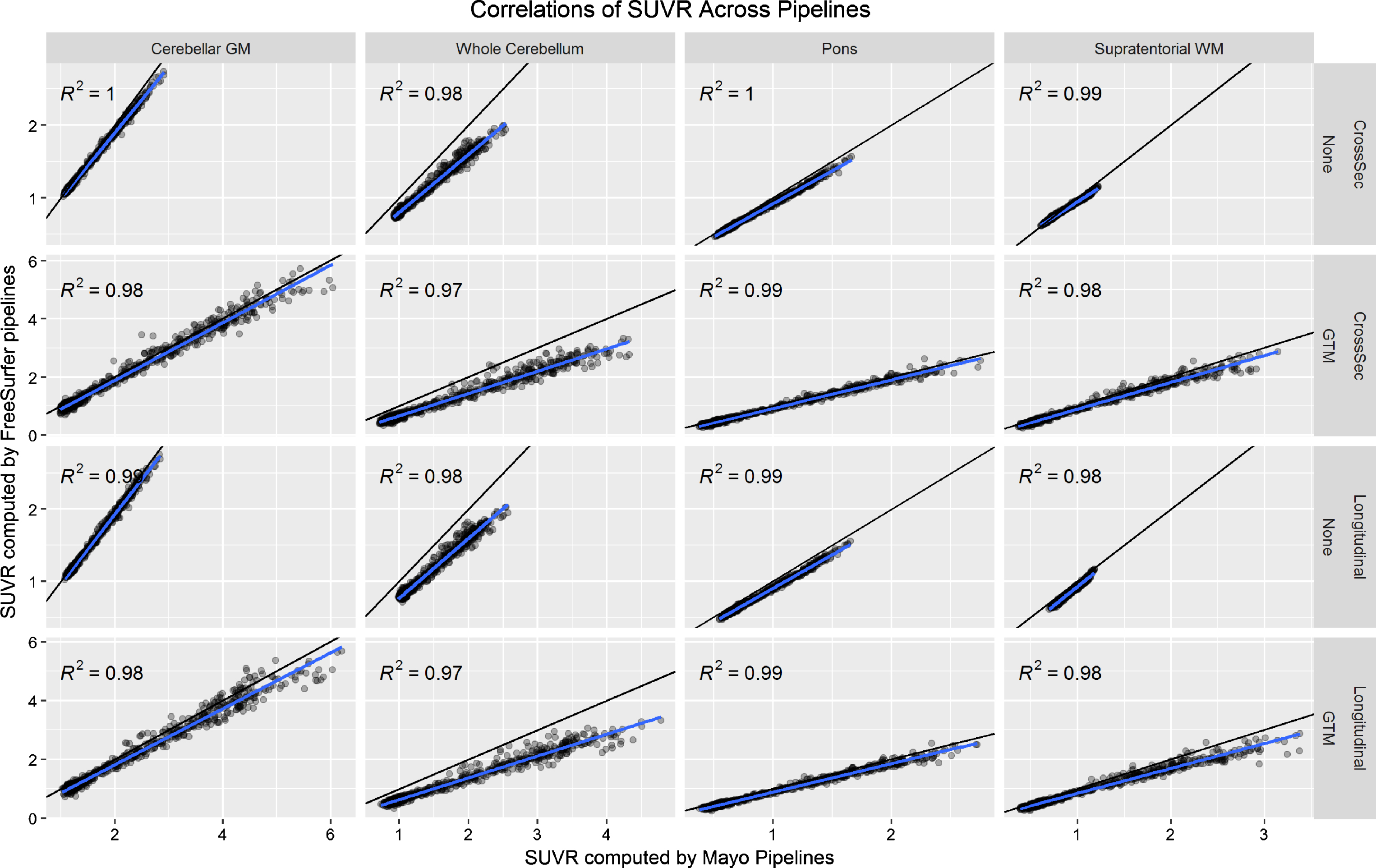
In Fig. 1, we plot correlations of SUVR values across the Mayo and FreeSurfer pipelines using each reference region with no PVC and GTM PVC (omitting the cerebellar crus reference region because this is not available in FreeSurfer). There were some systematic differences across the pipelines, which we attribute to systematic differences between segmentation methods and atlas region definitions. Even though these are fully-independent implementations, correlations between the two were very high (R2 > 0.97). We consider these high correlations strong evidence that neither implementation was faulty, effectively validating each other.
Fig.1
Relationship between PiB PET SUVR values as computed by the FreeSurfer versus Mayo pipelines. The black line indicates the identity line (y = x) and the blue line a fit from a linear regression model. Each plot gives the coefficient of determination (R2) from the regression model.
Coefficient of variation
We plot the results of our CV analysis in Fig. 2 as a function of pipeline, PVC method, and reference region. The cerebellar crus ROI and two/three-component PVC are unavailable with FreeSurfer’s mri_gtmpvc tool, so these combinations were omitted. Three-compartment PVC was also omitted for reference regions containing WM (whole cerebellum, pons, supratentorial WM), because this method removes signal in WM. Note that the Mayo pipelines use GTM PVC in the original Rousset style [13], while the FreeSurfer pipelines use the Symmetric GTM variant [23]. Based on the high correlations between them (Fig. 1), we refer to both as GTM PVC and compare them directly.
Fig.2
Coefficient of variation (CV) in PiB PET SUVR when using each combination of measurement pipeline, PVC, and reference region. CV was estimated from a linear mixed-effects model of log-transformed SUVR values using 3 timepoints of PiB PET scans (n = 278 subjects) with corresponding MRI. CVs with GTM PVC were consistently significantly larger (worse) than when using 2-compartment PVC or no PVC.
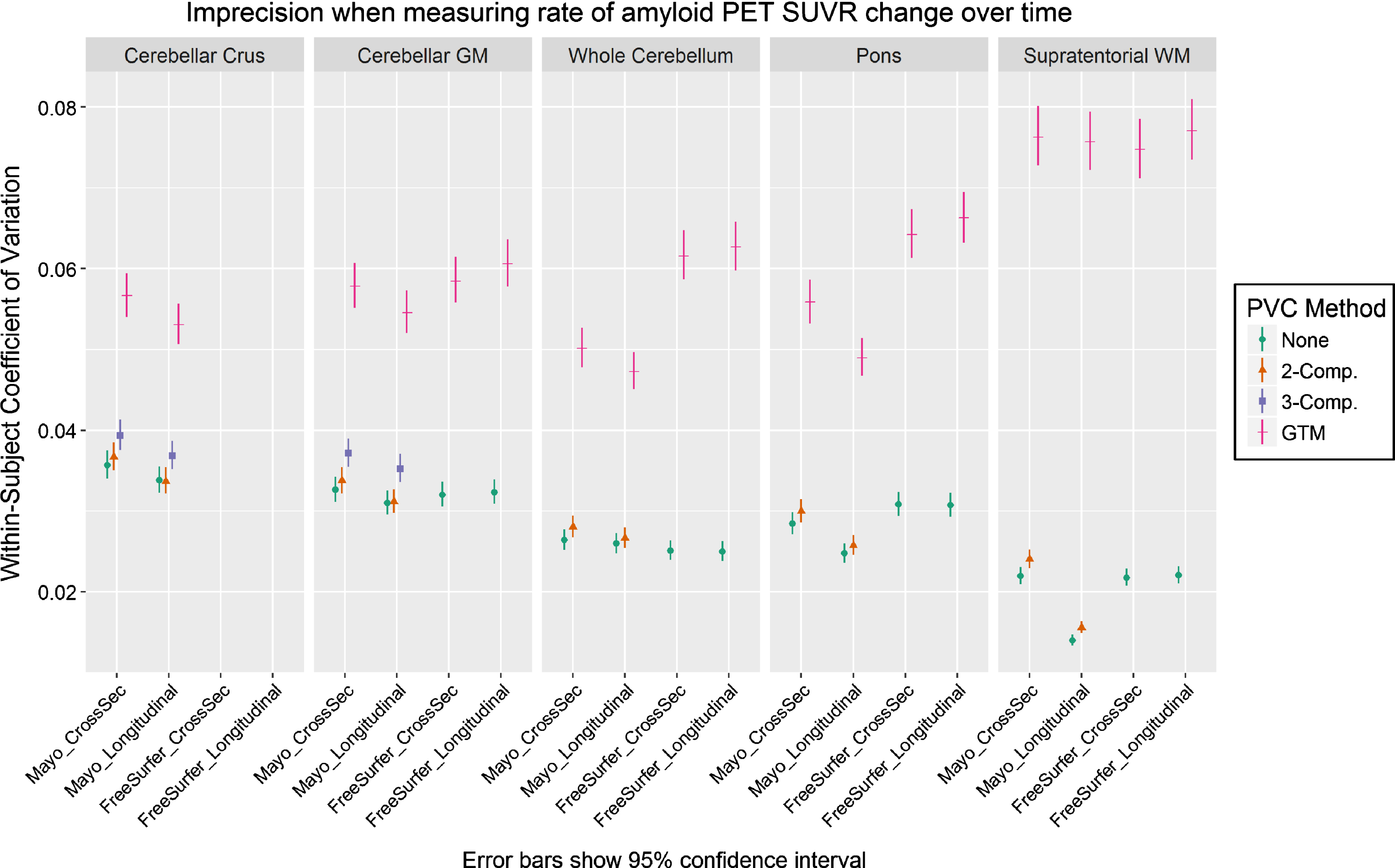
For all comparisons, serial GTM PVC SUVR measurements had appreciably greater CVs than corresponding voxel-based- and no-PVC measurements, which were relatively comparable with each other. Within otherwise-equivalent pipelines, the CV for GTM was always at least 50% greater than that for no-PVC or two-compartment PVC, and on-average it was more than twice as high. The CV for GTM was also at least 40% greater than all otherwise-equivalent pipelines using three-compartment PVC.
The longitudinal versions of each pipeline provided mixed results versus each corresponding cross-sectional variation, showing that their design features to stabilize serial values were minimally- or not effective under the tested conditions. Comparisons of Mayo versus FreeSurfer pipelines were also mixed. The (non-eroded) supratentorial WM reference region with two-compartment or no PVC performed best by this analysis, but this would be a flawed reference region choice because there is no correction for bleed-in of cortical signal, and there were no clear winners among the other reference regions.
Group-wise differences in slopes
In Fig. 3, we plot the results of our analysis comparing each method’s ability to detect a difference in the rate of amyloid increase between the clinically impaired and clinically unimpaired subject groups. We assume that a correctly-functioning method should show that the impaired group on-average accumulated amyloid faster than the unimpaired group, but the true magnitude of the difference in rates between these groups is unknown. Therefore, we consider all methods with a difference significantly >0 to be equivalently valid. We plot difference in annualized SUVR change as a percentage, rather than unscaled, to allow for comparison across methods and reference regions that have differing SUVR unit scales. For interested readers, we also provide this data in tabular form in Supplementary Table 1.
Fig.3
Difference between the annual rate of increase in PiB PET SUVR in clinically impaired versus that in clinically unimpaired subjects, when using each combination of measurement pipeline, PVC type, and reference region. Slopes for each group were assessed using a linear mixed-effects model of log-transformed SUVR values with separate fixed effect slopes and intercepts by impairment status. All methods showing differences > zero were considered equally plausible (we assume that amyloid should increase faster in impaired subjects, but the exact ground-truth difference is unknown). We plot difference in annualized SUVR change (y axis) as a percentage, rather than unscaled, to allow for comparison across methods and reference regions that have differing SUVR unit scales. Methods using GTM PVC produced group-wise differences that were larger but with much wider confidence intervals.
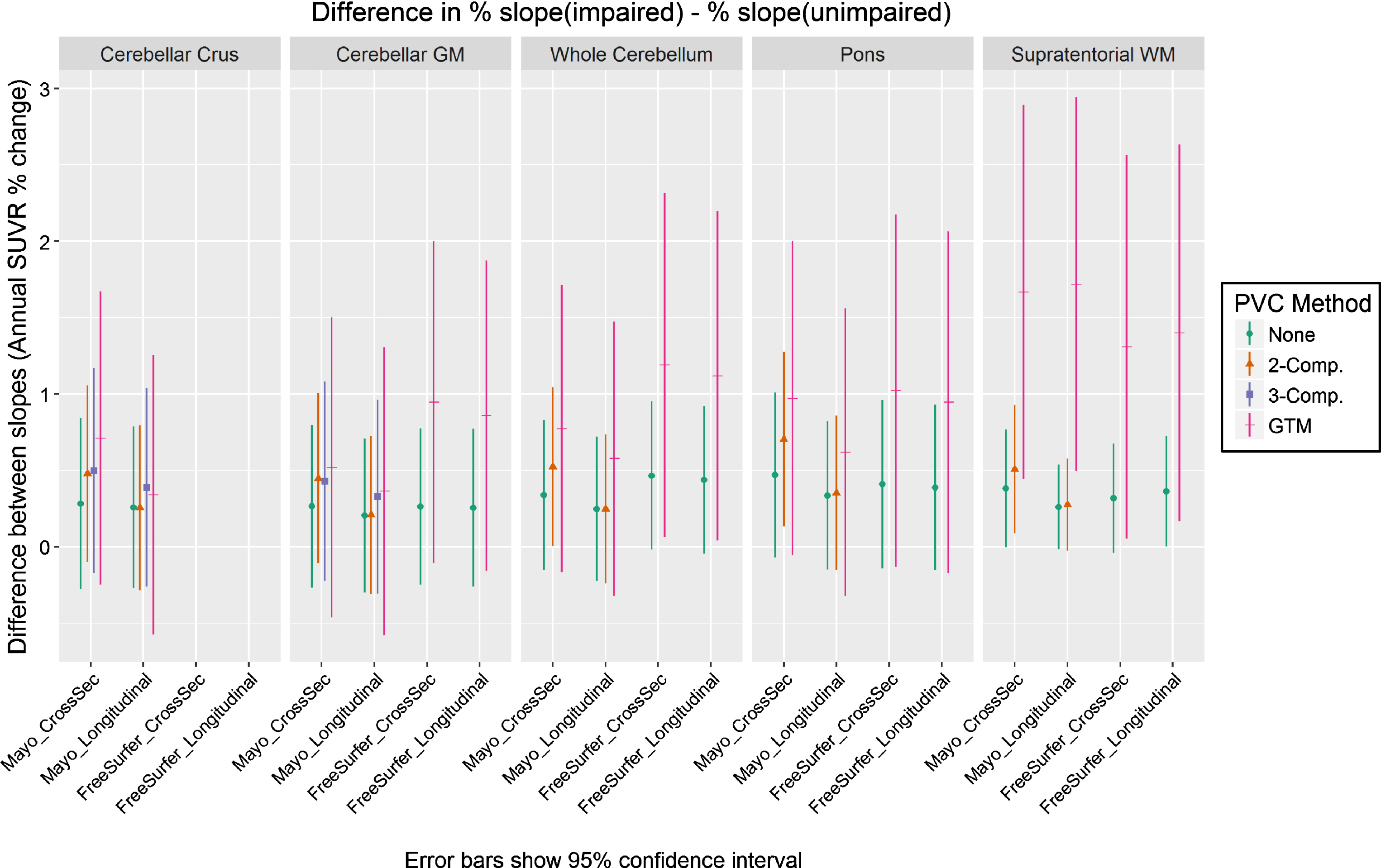
For most comparisons, group-wise differences were largest with GTM PVC and smallest with no PVC. Two-class PVC was generally in between GTM and no-PVC for cross-sectional pipelines, but orderings in longitudinal pipelines were mixed. However, the confidence intervals of these GTM PVC measurements were also wider due to their worse precision (explored in the previous section). The only methods whose confidence intervals excluded zero used either two-compartment or GTM PVC, but there were no significant differences across methods in their group-wise separation ability.
DISCUSSION
Discussion of results
The most significant and impactful finding of our study was that measurements of amyloid PET SUVR based on GTM PVC had an appreciably higher coefficient of variation compared to those based on more traditional (i.e., no-PVC or voxel-based PVC) methods (Fig. 2) and consequently GTM may not be appropriate for longitudinal studies where rates of change tend to be small and group-wise differences in rates of change tend to be subtle. PVC methods inherently amplify noise [13], so we were not surprised by this pattern. However, we were surprised by the magnitude of the worse precision of GTM PVC compared to two- or three-compartment PVC or no PVC. Correlations between partial volume corrected (as well as uncorrected) SUVR values using the independent Mayo and FreeSurfer pipelines were extremely high, suggesting that this finding is not the result of a quirk in a specific implementation of GTM. GTM’s relative instability was comparably large with both implementations, i.e., FreeSurfer’s symmetric GTM implementation did not produce more precise measurements than the Mayo pipelines’ traditional GTM. This data does not support the proposed benefits of symmetric GTM [23], but our comparison of these is not a direct one. Our measured CV when using the cerebellar gray matter reference without PVC was ≈3% (Fig. 2), which is smaller than previously reported measurements of PiB test-retest variability (8.0±7.0% in n = 6 AD, 4.4±4.2% in n = 6 controls) from back to back repeat scans [50].
Measurements using GTM PVC trended toward having the largest group-wise differences in annualized rates of SUVR increase (Fig. 3). We expected this ordering because PVC typically increases the dynamic range of output SUVR values when subjects have differing levels of atrophy, and GTM does this to a much greater magnitude than two- or three-compartment (for an example, see our companion cross-sectional analysis in the Supplementary Material). However, the increased noise of GTM PVC methods resulted in larger confidence intervals for group-wise differences, and differences between all methods in this comparison were not significant. Overall, this data suggests that the relative imprecision of serial measurements using GTM PVC is not outweighed by an increased power to detect group-wise differences.
Most methods did not detect any significant difference (confidence intervals excluding zero) in annualized rates of SUVR increase between the impaired and unimpaired subject groups (Fig. 3). To examine this, we computed the proportion of subjects in each group that were amyloid-positive at baseline according to a threshold of SUVR >1.42 using a cerebellar crus reference region with the Mayo cross-sectional pipeline [29]. Approximately 35% (35/99) of subjects in the impaired group were amyloid-negative at baseline (expected to have relatively-low rates of accumulation), and approximately 26% (46/179) of the unimpaired group were amyloid-positive (expected to have relatively-high rates of accumulation). Therefore, average rates should be higher in the impaired versus the non-impaired group. However, our finding that most methods did not differentiate between these clinically-characterized groups is expected given their overlap in expected amyloid trajectories. We did not define the groups using amyloid positivity because this would introduce circularity into the analysis, and because our goal is to compare methods which each used the same subject groupings with these same limitations (however, we did perform a separate analysis based on amyloid positivity in the Supplementary Material). Inclusion of our groupwise-separation metric is necessary to ensure that no methods have achieved reliability at the cost of removing all signal, but because of its limitations, we consider our coefficient of variation metric to be relatively far more important when comparing methods.
Although GTM PVC had a much larger coefficient of variation than the other measurement methods, CV differed only minimally or insignificantly between no PVC and the other, voxel-based methods (two- or three-compartment). Because these voxel-based methods can be used to correct for partial volume with minimal penalty in measurement stability, these results might suggest that their use should be encouraged when measuring change over time, if not generally. However, our study also found no significant improvements to group-wise differences by using the voxel-based methods, so our findings are mostly neutral regarding whether or not to use them for measuring amyloid change over time. Many studies have reported larger effect sizes when using PVC methods (for example, our corresponding cross-sectional analysis in the Supplementary Material), but it is unclear whether this increased study power comes from appropriately correcting for partial volume effects, or from other sources such as PVC techniques’ effectively multiplying PET data by MRI data and thus gaining power from MRI by combining both sources of information. In studies that analyze results from both MRI and PET, it is unknown whether partial volume corrected PET findings may be driven by the underlying MRI used in the correction, thus reducing the statistical independence of PET-driven findings from MRI-driven findings. One recent study showed that a set of PVC techniques similar to those in our study resulted in minimally decreased correlations between ante-mortem PiB PET scans and postmortem histological assessments of amyloid-β pathology [9], relative to no PVC. Those findings suggest that the biological mechanisms behind any improved effect sizes from using partial volume correction are unclear. Overall, more research is needed to determine the effects of PVC in amyloid PET imaging.
Strengths and limitations of current study
To our knowledge, this is the first study to compare the suitability of PVC methods specifically for longitudinal analysis in amyloid PET SUVR. We used a large sample (n = 278) of subjects with 3-timepoints each, allowing for more stable estimates of both within-person change and measurement error. We also used two fully-independent SUVR quantification pipelines for internal validation and to confirm that our comparison findings are intrinsic to the underlying methods rather than specific implementations. Each major pipeline also included a state-of-the-art longitudinal variant designed specifically to stabilize serial measurements, but these pipelines did not appreciably stabilize measurements and in particular did not increase precision in longitudinal GTM PVC measurements.
Our large dataset used a combination of multiple MRI and PET scanners, which can introduce additional variability versus smaller, single-scanner studies. To ensure that our conclusions were not due to inter-scanner differences, we also repeated our analyses using only the subset of subjects (n = 11) that retained a single pair of MRI+PET scanners for all three time points. All of our major findings were replicated at the trend level in this reduced subset, suggesting that inter-scanner differences did not significantly influence our findings, but the differences between methods were not significant due to the very-reduced sample size (data not presented).
This study compares only the major popular PVC algorithms. Many other methods and variants have publicly available implementations [8], but for space and practical reasons we must leave their comparisons for future work. It also uses only one amyloid PET tracer (PiB). We focused on amyloid because our quality metric is longitudinal precision and sufficiently large cohorts of serial amyloid PET are presently available. Future work will be needed to determine whether these findings also apply to other tracers, such as F-18 amyloid tracers, and to tau PET tracers (when sufficient longitudinal data becomes available).
A through technical exploration of possible tweaks and variations of GTM PVC is needed to understand specifically why it was less longitudinally stable versus other methods. For interested readers, in the Supplementary Material we present a short preliminary follow-up analysis including an additional variant that assumes non-brain regions have zero signal (as in the voxel-based methods), rather than treating them the same as any other regions (as in typical implementations of GTM). However, we must leave the necessary further exploration of mechanisms for GTM’s instability for future work. Our analysis included the symmetric variant of GTM designed to improve its noise properties (in the FreeSurfer pipelines), but this did not improve the stability of serial measurements over standard GTM (in the Mayo pipelines). We did not examine alternative methods of parcellating regions for GTM PVC (except for the one variant in the Supplementary Material, which had very mixed performance across differing reference regions). The GTM PVC method does not specify how regions may be parcellated, but it assumes that all signal in the PET image is explained by a combination of the modelled regions. Our study used brain parcellations that each (Mayo and FreeSurfer) included over 100 relatively-small cortical regions together with relatively large, homogeneous regions for WM, cerebrospinal fluid, and non-brain tissue; this reflects typical usage in recent studies, and the design of PETSurfer. This differs, however, from the original Rousset GTM validation that used a brain phantom with one region for caudate nucleus, one for putamen, one for globus pallidus, and another for all “background” voxels [13]. Similarly, the Symmetric GTM validation also used phantoms and simulations with relatively few regions [23]. It has been theorized that large matrices of regions may cause GTM’s matrix inversion to become unstable or ill-conditioned [10]. On the contrary, some studies have provided evidence that GTM PVC may perform better when smaller regions with more homogeneous signal are used [42]. Relatedly, it has also not been explored whether ROI definition should match those used for a desired analysis (e.g., one single cortical target region for amyloid versus correcting each individually and averaging regional values after PVC). We leave an exploration of these trade-offs between larger/smaller parcellations to future work.
Conclusions
Our findings suggest that increased within-person variability in GTM PVC may make it relatively unsuitable for computing measurements of within-person change over time from serial amyloid PET scans, and that advanced techniques designed to improve it for this purpose are not sufficient. We realize that traditional voxel-based PVC methods cannot provide corrections for spill-in and spill-out of signal between adjacent target and/or off-target regions, making it challenging to accurately estimate PET signal uptake in small focal regions without region-based methods. While our attempts to improve GTM for this purpose via longitudinal processing approaches were not sufficient, we hope that future developments may lead to an acceptable solution.
We stress that our primary findings are limited strictly to the longitudinal analysis context (an exploratory, retrospective cross-sectional analysis using the baseline data is also provided in the Supplementary Material). Serial imaging measurements reflect the accumulation of pathology over relatively short time frames and are intrinsically far smaller in magnitude than cross-sectional measurements that reflect accumulated pathology over the lifespan. For example, the average annual PiB PET SUVR increase in MCI and AD-Dementia subjects is approximately 0.05 SUVR units while the mean SUVR for this group is approximately 2.0. The annual rate of increase is approximately 2.5% of the cross-sectional average [15]. As a consequence of this difference in magnitudes, a far larger degree of imprecision is acceptable in cross-sectional measurements than in longitudinal change measurements.
In our serial PiB dataset, we observed coefficients of (unexplained) SUVR variation of ≈2–4% for two-compartment, three-compartment, or no PVC, and of ≈4–8% when using GTM PVC. Our CVs with a cerebellar gray matter reference and without PVC were ≈3%, which is smaller than previously reported measurements (8.0±7.0% in n = 6 AD, 4.4±4.2% in n = 6 controls) from back to back repeat scans [50]. However, these values should also be compared to the average annual PiB SUVR increase in PiB+ subjects, which is only ≈2.5% [15]. These numbers suggest that the field has a strong need to further identify and reduce sources of unwanted variation in serial amyloid, if not all serial PET SUVR measurements.
ACKNOWLEDGMENTS
The authors gratefully thank our funding sources that made this work possible: NIH grants R01 AG011378, R01 AG041851, U01 AG006786, P50 AG016574, R01 AG034676, R01 NS097495; Gerald and Henrietta Rauenhorst Foundation, Elsie and Marvin Dekelboum Family Foundation, Alexander Family Alzheimer’s Disease Research Professorship of the Mayo Clinic, Liston Award, Schuler Foundation, and Mayo Foundation for Medical Education and Research. We also thank Brad Kemp for his assistance with details of the nuclear medicine acquisitions.
Authors’ disclosures available online (https://www.j-alz.com/manuscript-disclosures/18-0749r1).
SUPPLEMENTARY MATERIAL
[1] The supplementary material is available in the electronic version of this article: http://dx.doi.org/10.3233/JAD-180749.
REFERENCES
[1] | Shidahara M , Thomas BA , Okamura N , Ibaraki M , Matsubara K , Oyama S , Ishikawa Y , Watanuki S , Iwata R , Furumoto S , Tashiro M , Yanai K , Gonda K , Watabe H ((2017) ) A comparison of five partial volume correction methods for Tau and Amyloid PET imaging with [18F]THK5351 and [11C]PIB. Ann Nucl Med 31: , 563–569. |
[2] | Thomas BA , Erlandsson K , Reilhac A , Bousse A , Kazantsev D , Pedemonte S , Vunckx K , Arridge S , Ourselin S , Hutton BF ((2012) ) A comparison of the options for brain partial volume correction using PET/MRI. 2012 IEEE Nuclear Science Symposium and Medical Imaging Conference Record (NSS/MIC). 10.1109/NSSMIC.2012.6551662. |
[3] | Harri M , Mika T , Jussi H , Nevalainen OS , Jarmo H ((2007) ) Evaluation of partial volume effect correction methods for brain positron emission tomography: Quantification and reproducibility. J Med Phys 32: , 108–117. |
[4] | Meltzer CC , Kinahan PE , Greer PJ , Nichols TE , Comtat C , Cantwell MN , Lin MP , Price JC ((1999) ) Comparative evaluation of MR-based partial-volume correction schemes for PET. J Nucl Med 40: , 2053–2065. |
[5] | Rullmann M , Dukart J , Hoffmann K-T , Luthardt J , Tiepolt S , Patt M , Gertz H-J , Schroeter ML , Seibyl J , Schulz-Schaeffer WJ , Sabri O , Barthel H ((2016) ) Partial-volume effect correction improves quantitative analysis of 18F-florbetaben β-amyloid PET scans. J Nucl Med 57: , 198–203. |
[6] | Bauer CM , Cabral HJ , Greve DN , Killiany RJ ((2013) ) Differentiating between normal aging, mild cognitive impairment, and Alzheimer’s disease with FDG-PET: Effects of normalization region and partial volume correction method. J Alzheimers Dis Parkinsonism 3: , 113. |
[7] | Erlandsson K , Buvat I , Pretorius PH , Thomas BA , Hutton BF ((2012) ) A review of partial volume correction techniques for emission tomography and their applications in neurology, cardiology and oncology. Phys Med Biol 57: , R119–R159. |
[8] | Thomas BA , Cuplov V , Bousse A , Mendes A , Thielemans K , Hutton BF , Erlandsson K ((2016) ) PETPVC: A toolbox for performing partial volume correction techniques in positron emission tomography. Phys Med Biol 61: , 7975–7993. |
[9] | Minhas DS , Price JC , Laymon CM , Becker CR , Klunk WE , Tudorascu DL , Abrahamson EE , Hamilton RL , Kofler JK , Mathis CA , Lopez OL , Ikonomovic MD ((2018) ) Impact of partial volume correction on the regional correspondence between in vivo [C-11]PiB PET and postmortem measures of Aβ load. Neuroimage Clin 19: , 182–189. |
[10] | Thomas BA , Erlandsson K , Modat M , Thurfjell L , Vandenberghe R , Ourselin S , Hutton BF ((2011) ) The importance of appropriate partial volume correction for PET quantification in Alzheimer’s disease. Eur J Nucl Med Mol Imaging 38: , 1104–1119. |
[11] | Meltzer CC , Leal JP , Mayberg HS , Wagner HNJ , Frost JJ ((1990) ) Correction of PET data for partial volume effects in human cerebral cortex by MR imaging. J Comput Assist Tomogr 14: , 561–570. |
[12] | Müller-Gärtner HW , Links JM , Prince JL , Bryan RN , McVeigh E , Leal JP , Davatzikos C , Frost JJ ((1992) ) Measurement of radiotracer concentration in brain gray matter using positron emission tomography: MRI-based correction for partial volume effects. J Cereb Blood Flow Metab 12: , 571–583. |
[13] | Rousset OG , Ma Y , Evans AC ((1998) ) Correction for partial volume effects in PET: Principle and validation. J Nucl Med 39: , 904–911. |
[14] | Su Y , Blazey TM , Snyder AZ , Raichle ME , Marcus DS , Ances BM , Bateman RJ , Cairns NJ , Aldea P , Cash L , Christensen JJ , Friedrichsen K , Hornbeck RC , Farrar AM , Owen CJ , Mayeux R , Brickman AM , Klunk W , Price JC , Thompson PM , Ghetti B , Saykin AJ , Sperling RA , Johnson KA , Scho PR , Buckles V , Morris JC , Benzinger TLS , Dominantly Inherited Alzheimer Network ((2015) ) Partial volume correction in quantitative amyloid imaging. Neuroimage 107: , 55–64. |
[15] | Jack CRJ , Wiste HJ , Lesnick TG , Weigand SD , Knopman DS , Vemuri P , Pankratz VS , Senjem ML , Gunter JL , Mielke MM , Lowe VJ , Boeve BF , Petersen RC ((2013) ) Brain β-amyloid load approaches a plateau. Neurology 80: , 890–896. |
[16] | Meltzer CC , Zubieta JK , Links JM , Brakeman P , Stumpf MJ , Frost JJ ((1996) ) MR-based correction of brain PET measurements for heterogeneous gray matter radioactivity distribution. J Cereb Blood Flow Metab 16: , 650–658. |
[17] | Klunk WE , Engler H , Nordberg A , Wang Y , Blomqvist G , Holt DP , Bergström M , Savitcheva I , Huang GF , Estrada S , Ausén B , Debnath ML , Barletta J , Price JC , Sandell J , Lopresti BJ , Wall A , Koivisto P , Antoni G , Mathis CA , Långström B ((2004) ) Imaging brain amyloid in Alzheimer’s disease with Pittsburgh Compound-B. Ann Neurol 55: , 306–319. |
[18] | Roberts RO , Geda YE , Knopman DS , Cha RH , Pankratz VS , Boeve BF , Ivnik RJ , Tangalos EG , Petersen RC , Rocca WA ((2008) ) The Mayo Clinic Study of Aging: Design and sampling, participation, baseline measures and sample characteristics. Neuroepidemiology 30: , 58–69. |
[19] | Petersen RC , Roberts RO , Knopman DS , Geda YE , Cha RH , Pankratz VS , Boeve BF , Tangalos EG , Ivnik RJ , Rocca WA ((2010) ) Prevalence of mild cognitive impairment is higher in men. The Mayo Clinic Study of Aging. Neurology 75: , 889–897. |
[20] | Iatrou M , Ross SG , Manjeshwar RM , Stearns CW ((2004) ) A fully 3D iterative image reconstruction algorithm incorporating data corrections. IEEE Nucl Sci Symp Conf Rec 4: , 2493–2497. |
[21] | Stearns CW , Fessler JA ((2002) ) 3D PET reconstruction with FORE and WLS-OS-EM. In IEEE Nuclear Science Symposium Conference Record IEEE, pp. 912–915. |
[22] | Herscovitch P , Auchus AP , Gado M , Chi D , Raichle ME ((1986) ) Correction of positron emission tomography data for cerebral atrophy. J Cereb Blood Flow Metab 6: , 120–124. |
[23] | Sattarivand M , Kusano M , Poon I , Caldwell C ((2012) ) Symmetric geometric transfer matrix partial volume correction for PET imaging: Principle, validation and robustness. Phys Med Biol 57: , 7101–7116. |
[24] | FreeSurfer wiki, FreeSurfer wiki: PETSurfer, Last updated 2016, Accessed on, 2016. |
[25] | Ashburner J ((2009) ) Computational anatomy with the SPM software. Magn Reson Imaging 27: , 1163–1174. |
[26] | Avants BB , Tustison NJ , Song G , Cook PA , Klein A , Gee JC ((2011) ) A reproducible evaluation of ANTs similarity metric performance in brain image registration. Neuroimage 54: , 2033–2044. |
[27] | Schwarz CG , Gunter JL , Ward CP , Vemuri P , Senjem ML , Wiste HJ , Petersen RC , Knopman DS , Jack CR ((2017) ) The Mayo Clinic Adult Lifespan Template: Better quantification across the lifespan. Alzheimers Dement 13: , P792. |
[28] | Jovicich J , Czanner S , Greve D , Haley E , Van Der Kouwe A , Gollub R , Kennedy D , Schmitt F , Brown G , MacFall J , Fischl B , Dale A ((2006) ) Reliability in multi-site structural MRI studies: Effects of gradient non-linearity correction on phantom and human data. Neuroimage 30: , 436–443. |
[29] | Jack CRJ , Wiste HJ , Weigand SD , Therneau TM , Lowe VJ , Knopman DS , Gunter JL , Senjem ML , Jones DT , Kantarci K , Machulda MM , Mielke MM , Roberts RO , Vemuri P , Reyes D , Petersen RC ((2017) ) Defining imaging biomarker cut points for brain aging and Alzheimer’s disease. Alzheimers Dement 13: , 205–216. |
[30] | Schwarz CG , Gunter JL , Wiste HJ , Przybelski SA , Weigand SD , Ward CP , Senjem ML , Vemuri P , Murray ME , Dickson DW , Parisi JE , Kantarci K , Weiner MW , Petersen RC , Jack CRJ ((2016) ) A large-scale comparison of cortical thickness and volume methods for measuring Alzheimer’s disease severity. Neuroimage Clin 11: , 802–812. |
[31] | Ashburner J , Friston KJ ((2005) ) Unified segmentation. Neuroimage 26: , 839–851. |
[32] | Avants BB , Epstein CL , Grossman M , Gee JC ((2008) ) Symmetric diffeomorphic image registration with cross-correlation: Evaluating automated labeling of elderly and neurodegenerative brain. Med Image Anal 12: , 26–41. |
[33] | Chen K , Roontiva A , Thiyyagura P , Lee W , Liu X , Ayutyanont N , Protas H , Luo JL , Bauer R , Reschke C , Bandy D , Koeppe RA , Fleisher AS , Caselli RJ , Landau S , Jagust WJ , Weiner MW , Reiman EM ((2015) ) Improved power for characterizing longitudinal amyloid-β PET changes and evaluating amyloid-modifying treatments with a cerebral white matter reference region. J Nucl Med 56: , 560–566. |
[34] | Fleisher AS , Joshi AD , Sundell KL , Chen Y-F , Kollack-Walker S , Lu M , Chen S , Devous MD , Seibyl J , Marek K , Siemers ER , Mintun MA ((2017) ) Use of white matter reference regions for detection of change in florbetapir positron emission tomography from completed phase 3 solanezumab trials. Alzheimers Dement 13: , 1117–1124. |
[35] | Landau SM , Fero A , Baker SL , Koeppe R , Mintun M , Chen K , Reiman EM , Jagust WJ ((2015) ) Measurement of longitudinal β-amyloid change with 18F-Florbetapir PET and standardized uptake value ratios. J Nucl Med 56: , 567–574. |
[36] | Schwarz CG , Senjem ML , Gunter JL , Tosakulwong N , Weigand SD , Kemp BJ , Spychalla AJ , Vemuri P , Petersen RC , Lowe VJ , Jack CR Jr. ((2017) ) Optimizing PiB-PET SUVR change-over-time measurement by a large-scale analysis of longitudinal reliability, plausibility, separability, and correlation with MMSE. Neuroimage 144: , 113–127. |
[37] | Schwarz CG , Gunter JL , Lowe V , Vemuri P , Senjem ML , Petersen RC , Knopman DS , Jack CR ((2017) ) Effects of using a novel longitudinal processing pipeline for measuring change over time in PiB PET. Alzheimers Dement 13: (7 Suppl), P455–P456. |
[38] | Avants BB , Yushkevich P , Pluta J , Minkoff D , Korczykowski M , Detre J , Gee JC ((2010) ) The optimal template effect in hippocampus studies of diseased populations. Neuroimage 49: , 2457–2466. |
[39] | Avants B , Cook PA , McMillan C , Grossman M , Tustison NJ , Zheng Y , Gee JC ((2010) ) Sparse unbiased analysis of anatomical variance in longitudinal imaging. Med Image Comput Comput Interv 6361: , 324–331. |
[40] | Schwarz CG , Jones DT , Gunter JL , Lowe VJ , Vemuri P , Senjem ML , Petersen RC , Knopman DS , Jack CR ((2017) ) Contributions of imprecision in PET-MRI rigid registration to imprecision in amyloid PET SUVR measurements. Hum Brain Mapp 38: , 3323–3336. |
[41] | Fox NC , Ridgway GR , Schott JM ((2011) ) Algorithms, atrophy and Alzheimer’s disease: Cautionary tales for clinical trials. Neuroimage 57: , 15–18. |
[42] | Baker SL , Maass A , Jagust WJ ((2017) ) Considerations and code for partial volume correcting [18F]-AV-1451 tau PET data. Data Br 15: , 648–657. |
[43] | Fischl B ((2012) ) Free surfer. Neuroimage 62: , 774–781. |
[44] | Reuter M , Schmansky NJ , Rosas HD , Fischl B ((2012) ) Within-subject template estimation for unbiased longitudinal image analysis. Neuroimage 61: , 1402–1418. |
[45] | Greve DN , Svarer C , Fisher PM , Feng L , Hansen AE , Baare W , Rosen B , Fischl B , Knudsen GM ((2014) ) Cortical surface-based analysis reduces bias and variance in kinetic modeling of brain PET data. Neuroimage 92: , 225–236. |
[46] | Freesurfer mailing list, [Freesurfer] Longitudinal surface analysis of PET data, Last updated 2016, Accessed on 2016. |
[47] | Gelman A , Hill J ((2006) ) Data Analysis Using Regression and Multilevel/Hierarchical Models, Cambridge University Press. |
[48] | Villemagne VL , Burnham S , Bourgeat P , Brown B , Ellis KA , Salvado O , Szoeke C , Macaulay SL , Martins R , Maruff P , Ames D , Rowe CC , Masters CL ((2013) ) Amyloid β deposition, neurodegeneration, and cognitive decline in sporadic Alzheimer’s disease: A prospective cohort study. Lancet Neurol 12: , 357–367. |
[49] | Braak H , Braak E ((1997) ) Frequency of stages of Alzheimer-related lesions in different age categories. Neurobiol Aging 18: , 351–357. |
[50] | Tolboom N , Yaqub M , Boellaard R , Luurtsema G , Windhorst AD , Scheltens P , Lammertsma AA , Van Berckel BNM ((2009) ) Test-retest variability of quantitative [11C]PIB studies in Alzheimer’s disease. Eur J Nucl Med Mol Imaging 36: , 1629–1638. |

