Counting synapses using FIB/SEM microscopy: a true revolution for ultrastructural volume reconstruction
1
Laboratorio de Circuitos Corticales, Centro de Tecnología Biomédica, Universidad Politécnica de Madrid, Madrid, Spain
2
Instituto Cajal, CSIC, Madrid, Spain
3
Carl Zeiss NTS GmbH, Oberkochen, Germany
The advent of transmission electron microscopy (TEM) in the 1950s represented a fundamental step in the study of neuronal circuits. The application of this technique soon led to the realization that the number of synapses changes during the course of normal life, as well as under certain pathological or experimental circumstances. Since then, one of the main goals in neurosciences has been to define simple and accurate methods to estimate the magnitude of these changes. Contrary to analysing single sections, TEM reconstructions are extremely time-consuming and difficult. Therefore, most quantitative studies use stereological methods to define the three-dimensional characteristics of synaptic junctions that are studied in two dimensions. Here, to count the exact number of synapses per unit of volume we have applied a new three-dimensional reconstruction method that involves the combination of focused ion beam milling and scanning electron microscopy (FIB/SEM). We show that the images obtained with FIB/SEM are similar to those obtained with TEM, but with the advantage that FIB/SEM permits serial reconstructions of large volumes of tissue to be generated rapidly and automatically. Furthermore, we compared the estimates of the number of synapses obtained with stereological methods with the values obtained by FIB/SEM reconstructions. We concluded that FIB/SEM not only provides the actual number of synapses per volume but it is also much easier and faster to use than other currently available TEM methods. More importantly, it also avoids most of the errors introduced by stereological methods and overcomes the difficulties associated with these techniques.
In the cerebral cortex there are two main morphological types of synapses, Gray’s type I and type II synapses (Gray, 1959
) that correspond to the asymmetric and symmetric types of Colonnier, respectively (Colonnier, 1968
; see also, Colonnier, 1981
; Peters, 1987
; Peters et al., 1991
; Peters and Palay, 1996
). In general, asymmetric synapses are considered to be excitatory (glutamatergic) and symmetric synapses inhibitory (GABAergic). Moreover, asymmetric synapses are much more abundant (75–95% of all neocortical synapses) than symmetric synapses (5–25%: for reviews, see Houser et al., 1984
; White, 1989
; DeFelipe and Fariñas, 1992
; DeFelipe et al., 2002
). Therefore, understanding the distribution, size and proportion of the two major cortical types of synapses is extraordinarily important in terms of function.
Considerable effort has been dedicated to define methods that accurately estimate the number of synapses in the cerebral cortex, as well as the changes that take place during the course of normal life, and under pathological or experimental conditions. As a result, stereological methods have been developed to estimate the three-dimensional characteristics of synapses from two-dimensional observations, and to estimate their size and number in a given volume of tissue. Two of these stereological methods have been commonly used, one of which is a size-frequency method based on the number of synaptic profiles per unit area and their average cross-sectional length in ultrathin sections of tissue (Colonnier and Beaulieu, 1985
). The other technique is the disector method, that is based on the number of synaptic profiles that are present in a reference section but that disappear in another section separated by a known distance (Sterio, 1984
).
Both methods rely on the analysis of a limited number of single sections and thus, the estimate of the number of synapses per unit volume may vary according to the sampling methods used in a particular study (DeFelipe et al., 1999
). In addition, there is no general consensus regarding sampling procedures or the criteria to identify synapses. As a consequence, there are often discrepancies in the results obtained in different laboratories and they can be difficult to compare. In this context, the ideal approach would be to directly analyze samples reconstructed from serial sections. This can be achieved by conventional serial-section transmission electron microscopy (TEM), but this is a time consuming and technically demanding task, mainly due to the difficulties in obtaining large numbers of correlative serial sections (see for example Harris et al., 2006
; Hoffpauir et al., 2007
). To overcome these problems, methods have been developed that avoid the need for ultrathin sectioning, such as serial section electron tomography (Soto et al., 1994
). Other techniques facilitate the collection of serial ultrathin sections (Hayworth et al., 2006
), or allow ultrathin sections to be studied under a scanning electron microscope (SEM) by back-scattered electron imaging (Kasthuri et al., 2007
; Micheva and Smith, 2007
; Smith, 2007
). Finally, there are methods in which sections are not used at all, but rather serial images are taken by back-scattered electron-SEM from the block face after slices are sequentially removed either with a diamond knife (Denk and Horstmann, 2004
) or by means of a focused ion beam (FIB: Langford, 2006
; Knott et al., 2008
; see also reviews in Briggman and Denk, 2006
; Smith, 2007
; Helmstaedter et al., 2008
).
Block face imaging methods avoid the loss and deformation of sections that are common when images are taken from serial sections. Indeed, the alignment of serial images is easier since the drift between successive sections is minimal. Furthermore, the serial milling of the block surface and image acquisition can be fully automated when using combined FIB/SEM, which allows large volumes of tissue to be studied without the need for any mechanical interaction with the sample. In this study we have used this new technology to show that the ultrastructural images are comparable in quality and resolution to those obtained with the conventional TEM, with none of the debris or artifacts generated by previous methods. More specifically, we have managed to solve the critical issue of unequivocally identifying asymmetric and symmetric synapses, and we can count them directly within a tissue volume of known size, thereby eliminating the need to estimate the number of synapses per unit volume from two-dimensional samples. We have also compared this technique with the more commonly used disector and size-frequency methods. Although the present study has focused on the cerebral cortex, what follows could be applied in general to other regions of the brain.
Tissue Preparation
Four 26-day-old C57 mice were administered a lethal intraperitoneal injection of sodium pentobarbital (40 mg/kg) and they were intracardially perfused at room temperature with saline solution, and then with 2% paraformaldehyde and 2.5% glutaraldehyde in 0.1 M sodium phosphate buffer (PB), pH 7.4, containing 0.02 M CaCl2. The brains were extracted from the skull and post-fixed at 4°C overnight in the same solution. They were then washed in PB and sectioned in a vibratome (150 μm thickness). Selected sections were osmicated for 1 h at room temperature in PB containing 1% OsO4, 7% glucose and 0.02 M CaCl2. After washing in PB, the sections were stained for 30 min with 1% uranyl acetate in 50% ethanol at 37°C, and they were then dehydrated and flat embedded in Araldite (DeFelipe and Fairén, 1993
). Embedded sections were glued onto a blank Araldite block and trimmed. In order to select the region of interest, several semithin sections (1–2 μm of thickness) were obtained from the surface of the block and stained with toluidine blue. All animals were handled in accordance with the guidelines for animal research set out in the European Community Directive 86/609/EEC and all procedures were also approved by the local ethics committee of the Spanish National Research Council (CSIC).
Focused Ion Beam Milling and the Acquisition of Serial Scanning Electron Microscopy Images
The blocks containing the embedded tissue were glued onto a sample stub using conductive silver paint (AGAR Scientific Ltd., Stansted, Essex, UK). All the surfaces of the blocks, except that to be studied (the top surface), were covered with silver paint to prevent charging the resin. The stubs with the mounted blocks were then placed into a sputter coater (Emitech K575X, Quorum Emitech, Ashford, Kent, UK) and the top surface was coated with a 10–20 nm thick layer of gold/palladium to facilitate charge dissipation.
The three-dimensional study of the samples was carried out using a combined FIB/SEM microscope (Crossbeam® Neon40 EsB, Carl Zeiss NTS GmbH, Oberkochen, Germany). This instrument combines a high resolution field emission SEM column (Gemini® column, Carl Zeiss NTS GmbH, Oberkochen, Germany) with a focused gallium ion beam which permits material to be removed from the sample surface on a nanometer scale. Regions of the neuropil were chosen on the surface of the tissue block for 3D analysis. A protective layer of carbon was deposited on top of the area to be analyzed using an ion beam with a 30-kV acceleration potential. Using a 10-nA ion beam current, a first coarse cross-section was milled as a viewing channel for SEM observation. The exposed surface of this cross-section was fine polished by lowering the ion beam current down to 200 pA. Subsequently, layers from the fine polished cross-section were serially milled by scanning the ion beam parallel to the surface of the cutting plane using the same ion beam current. To mill each layer, the ion beam was automatically moved closer to the surface of the cross-section by preset increments of 18.9 nm, which corresponded to the thickness of the layers. This layer thickness was verified by sectioning the reconstructed stack of images perpendicular to the original cutting plane. These reconstructed images were compared to the original SEM images and they displayed no evidence of distortions or apparent jumps in the thickness of the layers. The section thickness was also verified independently by measuring the diameter of mitochondria according to the method described by Fiala and Harris (2001a
,b
). When tissue shrinkage was taken into account (see below), the mean thickness of the layers was corrected to19.9 nm.
After the removal of each slice, the milling process was paused and the freshly exposed surface was imaged with a 2-kV acceleration potential using the in-column energy selective backscattered electron detector (EsB). A 30-μm aperture was selected for imaging and the retarding potential of the EsB grid was 1500 V. The milling and imaging processes were continuously repeated and long series of images were acquired in a fully automated procedure. For this study, we obtained images of 2048 × 1536 pixels, at a resolution of 3.7 nm per pixel, thereby covering an area of 7.577 × 5.683 μm before correction for shrinkage. Under these conditions each milling/imaging cycle took approximately 4 min. Samples up to a size of a 10-cm wafer, with a height up to 4 cm, can be loaded via a load-lock and they can be completely accessed.
Alignment and Visualization of Serial Images: Construction of the Counting Volume
The alignment (registration) of the serial microphotographs was performed with the ImageJ software (W. Rasband, National Institutes of Health)
1
, taking advantage of the turboreg and stackreg plug-ins (Ph. Thévenaz, école Polytechnique Fédérale de Lausanne)
2
. The resulting stack of serial sections was then cropped and further studied with the Reconstruct software (Fiala, 2005
). The final rendering of the 3D objects was made with Blender
3
. An unbiased counting frame that represented 32.5 μm2 (36.22 μm2 after correction for shrinkage, see below) was drawn on each of the microphotographs (Figures 1
A,B). To extend the counting frame to three dimensions, one section near the beginning of the series was considered as an acceptance plane, while another section near the end of the series was considered as an exclusion plane, thereby forming an unbiased counting brick bound by three acceptance planes and three exclusion planes (Howard and Reed, 2005
). All synaptic profiles that were fully contained in the brick or that intersected any of the acceptance planes and did not intersect any of the exclusion planes were counted (Figures 1
C,D). In this way, objects were counted within a regular rectangular prism of known dimensions: the height and width corresponded to the dimensions of the counting frame drawn on each microphotograph, while the length was the result of multiplying the number of sections by the mean section thickness.
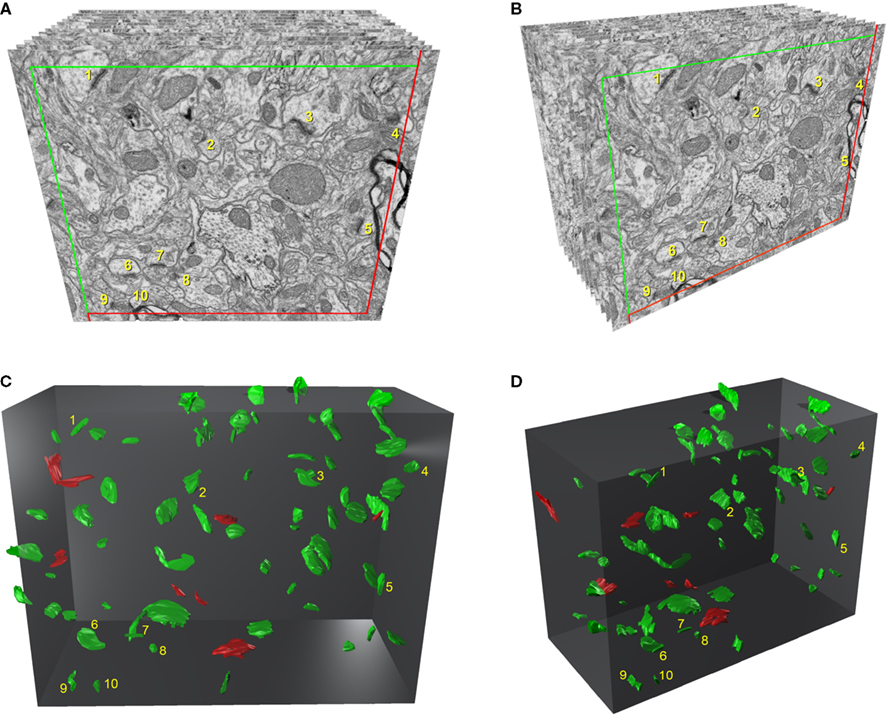
Figure 1. Three-dimensional representation of a stack of serial sections and the synaptic profiles that appear in the corresponding counting brick. (A) and (B) show a stack of serial sections, slightly rotated counter-clockwise through the vertical axis in (B). Only 12 sections are shown out of the 115 that compose the complete stack. An unbiased counting frame was drawn on each section, taking the green and the red lines as the acceptance and exclusion boundaries, respectively. To extend the counting frame to three dimensions, the front section was considered as an acceptance plane and the last section as an exclusion plane. Thus, synaptic profiles (contours of the synaptic membrane densities) were counted inside an unbiased counting brick bound by three acceptance planes (top, left and front) and three exclusion planes (right, bottom and back). As an example, the 10 synaptic profiles that appeared in the first section (acceptance plane), without intersecting any of the exclusion planes, have been numbered from 1 to 10 in (A) and (B). The counting frame measured 6.86 × 5.28 μm after correction for tissue shrinkage. In (C) and (D) the counting brick and the three dimensional reconstructions of synaptic profiles have been rendered. Green objects represent asymmetric synaptic profiles and red objects symmetric synaptic profiles. All the objects shown were inside the counting brick or intersected one of the acceptance boundaries, without intersecting any of the exclusion planes. Numbered objects correspond to the same synaptic profiles shown in (A) and (B). Note that every object can be individually identified and localized in the 3D space.
Brain tissue shrinks during processing for electron microscopy, especially during osmication and plastic embedding. To estimate the shrinkage in our samples we measured the surface area and thickness of the vibratome sections with Stereo Investigator (MBF Bioscience, Williston, VT, USA), both before and after they were processed for electron microscopy (Oorschot et al., 1991
). The surface area after processing was divided by the value before processing to obtain an area shrinkage factor (p2) of 0.897. The linear shrinkage factor for measurements in the plane of the section (p) was therefore 0.947. The shrinkage factor in the z-axis was 0.951. All distances measured were corrected to obtain an estimate of the pre-processing values.
Criteria for the Identification and Counting of Synapses
A synapse is recognized according to well-established criteria (e.g., see Colonnier, 1981
; Peters et al., 1991
; Peters and Palay, 1996
). Thus, a structure is identified as a synapse when the following elements are clearly recognized: densities on the cytoplasmic faces in the pre- and post-synaptic membranes; named synaptic membrane densities; synaptic vesicles in the pre-synaptic axon terminal adjacent to the pre-synaptic density; and a synaptic cleft, although this last element may not be visible if sectioned obliquely or frontally (en face). In general, three kinds of structural units have been used to count synapses (see Mayhew, 1996
, for a review): the terminal boutons; the total apposition zones; and the synaptic membrane densities, whose identification is commonly associated with other structural characteristics. Synaptic membrane densities are the units most commonly used for counting of synapses. In the present study we have adopted these counting units when they were accompanied by synaptic vesicles near the pre-synaptic density, and regardless of the angle of section at which the synaptic junctions were viewed (that is, whether a synaptic cleft was evident or not).
There is a general consensus for classifying cortical synapses into asymmetric (or type I) and symmetric (or type II) synapses. The main characteristic distinguishing these synapses is the prominent or thin post-synaptic density, respectively (Gray, 1959
; Colonnier, 1968
, 1981
; Peters, 1987
; Peters et al., 1991
; Peters and Palay, 1996
). Nevertheless, in single sections the synaptic cleft and the pre- and post-synaptic densities are often blurred if the plane of the section does not pass at right angles to the synaptic junction. The en face view is the most extreme case when the plane of section is parallel to the plane of the synaptic junction. For this reason, uncharacterized synapses are sometimes included in counts as asymmetric and symmetric types, according to the relative frequency of both types of synapses estimated by those already classified (see Discussion). Since synaptic junctions were fully reconstructed in the present study, all of them could be classified as asymmetric or symmetric.
Direct Quantification of Synapses from Stacks of Serial Sections
Using the Reconstruct software, we manually traced the contours of the synaptic membrane densities that appeared within the three-dimensional counting frame. For any given synapse, these contours comprised both the pre- and post-synaptic densities. Since they appeared in consecutive serial sections, the densities belonging to each individual synapse could be reconstructed in three-dimensions. Thus, each synapse was classified as asymmetric or symmetric and it was given a unique identification number (Figure 1
). Since the volume of each stack of sections was known, the number of synapses per unit volume was calculated directly by dividing the total number of synapses counted by the volume of the three-dimensional counting frame.
Thus, synaptic profiles were considered as 3D objects whose contours or traces appeared in several consecutive sections. Special attention was paid to the fact that some of these traces could intersect one of the acceptance or exclusion planes while others might not. The intersection of a single trace with one of the acceptance or exclusion planes was sufficient for the whole 3D object to be counted or not, respectively.
Estimation of the Number of Synapses by the Disector Method
Once the individual synaptic densities had been identified and their profiles traced, the sections in which they appeared were recorded with the Reconstruct software. The disector method is based on counting the profiles that are present in a given section (the reference section) and that disappear in another section (the look-up section) located at a known distance in the z-axis. The number of synaptic profiles that were present in the reference section but not in the look-up section (ΣQ−) was counted in each pair of images within the unbiased counting frame (Gundersen, 1977
). The number of synapses per unit volume (NV) was then calculated using the formula NV = ΣQ−/ah, where a is the area of the unbiased counting frame and h is the distance between the two sections.
Usually after one disector is calculated, the top and bottom microphotographs are swapped and used as the new reference and look-up sections. Thus, any given pair of sections yields two estimates (Gundersen et al., 1988a
). Since the presence or absence of synaptic profiles in each section was already defined by direct counting, all possible disectors (that is disectors using all possible combinations of pairs of sections at different distances) were calculated with the help of a worksheet. However, not all disectors were useful to estimate the number of synapses, since the distance between the sections (h) was too far in most cases, given that it should not exceed 1/4 to 1/3 the mean particle length (see below). Thus, only disectors where h = 3 times the section thickness were finally used. Having selected the appropriate h value for disectors, we simulated different sampling protocols, randomly choosing different numbers of section pairs from the stacks.
Estimation of the Number of Synapses by the Size-Frequency Method
Synaptic junctions were counted in each single section within the unbiased counting frame, and using the same profiles that were previously traced for the direct quantification of synapses and for the disector method. These profiles comprised the pre- and post-synaptic membrane densities of each synaptic junction. In order to measure the cross-sectional lengths of the synaptic junctions, each profile was first skeletonized using the ImageJ program. This procedure automatically converts any profile into a single longitudinal line that runs along the entire length of the profile. These lines were then measured with ImageJ. The number of synapses per unit volume (NV) was estimated using the formula NV = NA/d, where NA is the number of synaptic junctions per unit area and d, the mean cross-sectional length of the synaptic junctions (Colonnier and Beaulieu, 1985
). Like the disector method, the size-frequency method is usually performed on a limited number of sections. However, since we had already traced all the synaptic profiles in each section for the direct quantification, we applied the size-frequency method to all the sections in each stack. Afterwards, we also simulated different sampling protocols randomly choosing different numbers of sections.
Visualization, Identification and Classification of Synapses
Once the gray scale was inverted, the appearance of cortical tissue in the SEM images formed by back-scattered electrons was very similar to the microphotographs obtained by conventional TEM. At the resolution used (3.7 nm/pixel), the appearance of cell membranes and intracellular structures such as microtubules, neurofilaments, vesicles, cisternae, synaptic specializations, and mitochondria, were comparable to the images obtained with TEM, with the exception of myelin sheaths, that appeared to be darker and lacked fine detail under the conditions we used (Figure 2
). At the low imaging acceleration potential used (2 kV), the electron beam did not appear to cause any damage to the ultrastructure at the surface of the block when compared to conventional TEM images. Furthermore, the same block surface could be imaged several times (up to 10 times) with no noticeable alterations.
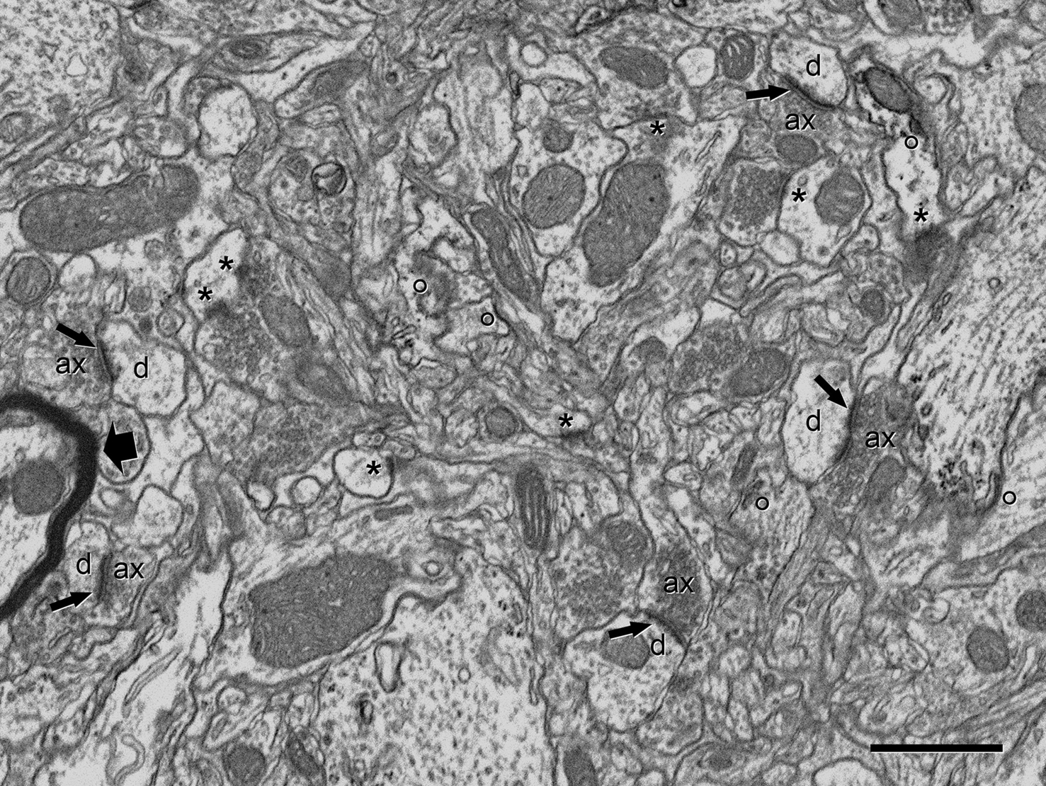
Figure 2. Panoramic view of the neuropil obtained in backscattered electron imaging mode. The high quality of the image is comparable to the images obtained with TEM. Intracellular structures such as filaments, vesicles, cisternae or mitochondria can be identified. Some axon terminals (ax) establish clearly identifiable asymmetric synapses (arrows) with dendritic spines (d). Other membrane densities could only be unambiguously identified as asymmetric or symmetric synaptic densities (asterisks), or non-synaptic densities (circles), when the neighboring serial sections were studied. The myelin sheath to the left of the figure (thick arrow) is very dark and its laminar structure cannot be resolved at this resolution. Scale bar, 1 μm.
The identification of synapses as well as their classification as asymmetric or symmetric was readily achieved in single sections (Figure 3
), or through their visualization in serial sections (Figure 4
, Supplemental Videos 1 and 2). When synapses were perforated, the examination of serial sections (Figure 5
) and three-dimensional reconstructions (Figure 6
) greatly facilitated the interpretation of images. Even when the synaptic junction was sectioned en face (Figure 7
), it was possible to estimate the approximate thickness of the synaptic densities, or to digitally reslice the stack of images through a different plane of section (Figure 8
), thereby allowing us to classify the synapse as asymmetric or symmetric. Therefore, if the interpretation of a synaptic junction was doubtful in a given section, it was clarified by studying the adjacent sections. In this way, individual synapses could not only be easily counted, but their size and shape, as well as their position within the sampled three-dimensional space, could be clearly visualized in the reconstructions (Figures 1 and 6
). The post-synaptic element could also be identified for each individual synapse as a dendritic spine or shaft (Figure 4
, Supplemental Videos 1 and 2). Although we chose a 3.7-nm/pixel resolution in this study, synapses were also readily identified at 4.3 nm/pixel. Synaptic densities were still visible at much lower resolutions (up to 8 nm/pixel) although they were blurred and with insufficient detail to recognize smaller structures such as synaptic vesicles.
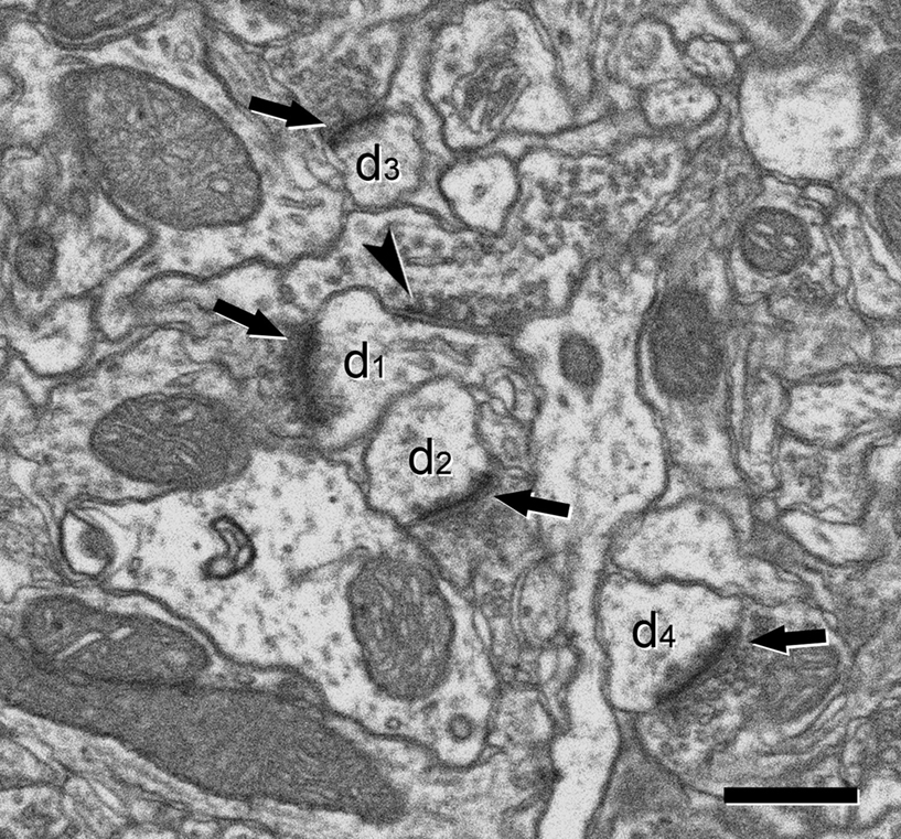
Figure 3. Ultrastructural appearance of asymmetric and symmetric synapses. Four asymmetric synapses (arrows) and one symmetric synapse (arrowhead) can be identified on four dendritic spines (d1 to d4). Asymmetric synapses show a thick post-synaptic density. The symmetric synapse has a thin post-synaptic density, very similar to the pre-synaptic density, and it is located on the neck of a dendritic spine (d1). Scale bar, 500 nm.
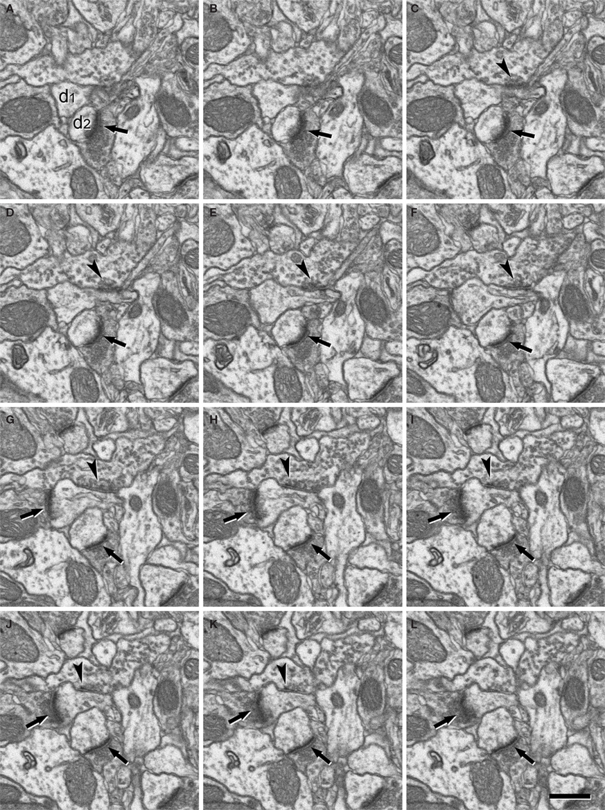
Figure 4. Serially sectioned symmetric and asymmetric synapses. (A-L) Consecutive serial sections focused on two of the asymmetric synapses (arrows) and the symmetric synapse (arrowheads) shown in Figure 3
. These three synapses are established on two dendritic spines, labeled d1 and d2 in section (A). The different thickness between the pre- and post-synaptic densities is especially evident for the asymmetric synapses when they are sectioned perpendicular to the membranes and the synaptic cleft is visible, as in sections (H) or (J) for the synapse on d1 and (E) to (L) for the synapse on d2. The symmetric synapse can be identified in sections (C) to (K) (arrowheads). Its synaptic cleft is visible in sections (F) to (K), where it is possible to appreciate that the pre- and post-synaptic densities are about the same thickness. Section (H) is shown at a higher magnification in Figure 3
. Section thickness, 19.9 nm. Scale bar, 500 nm.
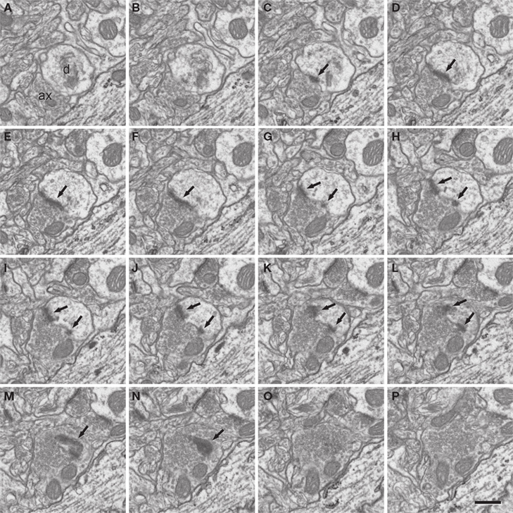
Figure 5. A perforated synapse serially sectioned. (A-P) In this series of sections only every second section has been represented. The synaptic contact (arrows) is established between an axon terminal that contains numerous synaptic vesicles and a dendritic spine [ax and d, respectively, in (A)]. Although the section plane appears to be oblique with respect to the synaptic junction, the synaptic cleft is partially visible in sections (E) and (F). This synapse can be identified as asymmetric on the basis of the prominent post-synaptic density evident in sections (C) to (N). Due to the fact that the synaptic junction is ring-shaped, there are two densities in sections (G) to (L). The examination of serial sections greatly facilitates the correct interpretation of this synapse as a perforated asymmetric synapse. For example, if only single sections were used, the sections in which the synaptic junction has been cut en face [(M) and (N)] would have been difficult to interpret. A three dimensional reconstruction of this synapse is represented in Figure 6
. Section thickness, 19.9 nm. Scale bar, 500 nm.
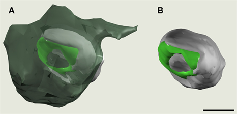
Figure 6. Three dimensional reconstruction of a perforated synapse. The synapse reconstructed here is the same that is shown in Figure 5
. In (A), the axon terminal (dark green) has been made semitransparent to permit the visualization of the dendritic spine head (light gray). The synaptic junction has been represented in light green. In (B), the axon terminal has been removed to better visualize the synaptic junction. The pre-synaptic terminal appears larger as an effect of the perspective. Scale bar, 500 nm.
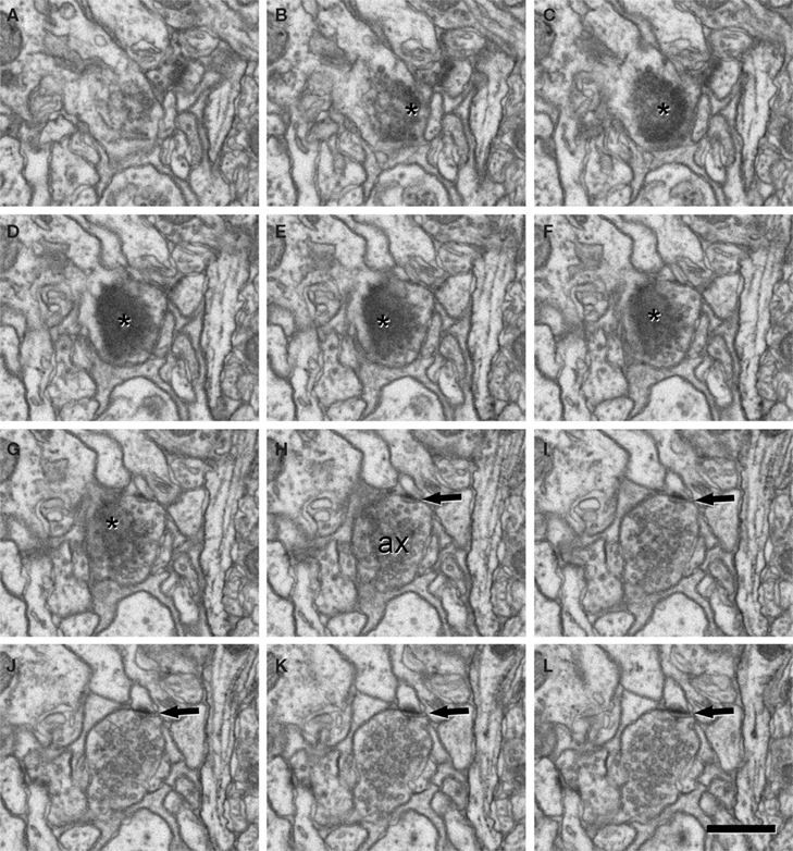
Figure 7. A synapse sectioned en face. (A-L) A series of sections to illustrate a synapse when the plane of section is almost completely parallel to the synaptic junction and thus, the pre- and post-synaptic densities, as well as the synaptic cleft, cannot be identified independently. Since the synaptic junction (asterisks) appears in sections (B) to (G), it apparently has a total thickness of about 100–120 nm (the individual section thickness was 19.9 nm). Although this thickness comprises both the pre- and post-synaptic densities and the synaptic cleft, the total thickness is prominent enough to suggest that it is an asymmetric synapse (the pre-synaptic membrane specialization and the synaptic cleft would account for about 40–50 nm). This could be confirmed because in the last four sections of the series, the pre-synaptic element [ax in (H)], characterized by the presence of numerous synaptic vesicles, establishes a small synapse that is clearly asymmetric (arrows). Scale bar, 500 nm.

Figure 8. A synapse digitally resliced trough a perpendicular plane of section. The synapse presented in (A) is the same that is shown in Figure 7
E. Using the ImageJ software (see text) a stack of 50 sections containing the synapse was digitally resliced through a plane perpendicular to the original plane of section. Thus, the synapse that was previously sectioned en face in (A) was sectioned transversally in (B) to (E). The lines on (A) indicate the position and orientation of the four selected sections shown in (B) to (E). The synaptic junction can be identified as a dense gray profile in (B) to (E) (asterisks). Although the pre and post-synaptic densities and the synaptic cleft cannot be individually resolved, the prominent thickness of the density (asterisks) strongly suggests that it is an asymmetric synapse. Thanks to the tilted angle of section (13°), a nearby asymmetric synapse can also be identified in (D) (arrow). This small synapse is the same that has already been shown in Figure 7
(H) to (L) where it can also be easily identified as an asymmetric synapse. The apparent loss of image quality in (B) to (E) is due to the fact that resolution in z-axis is limited by the section thickness of 19.9 nm. Scale bar, 500 nm.
The availability of long series of sections also facilitated the visualization and analysis of other elements in the neuropil. For example, neuronal and glial processes were easily followed in successive serial sections, as well as their branching processes. Dendritic spines could also be identified and traced up to their dendritic trunk. Individual mitochondria could be followed for several microns and surprisingly, we found that many dendrites had a single, long mitochondrion (Supplemental Video 1).
Direct Quantification vs the Disector and Size-Frequency Methods
Using the direct quantification method within an unbiased counting brick we could count the exact number of synapses within that volume. Since the dimensions of the brick were known, we could obtain a direct estimate of the number of synapses per unit volume. Once this value was defined, we compared it with the estimates obtained by the disector and size-frequency methods using different sampling protocols.
When applying the disector method, we first tried to determine the h value to be used (the distance between the reference and look-up sections). Theoretically, the estimation of object numbers with the disector is not influenced by section thickness, provided it does not exceed 1/4 to 1/3 the mean particle length (Gundersen et al., 1988a
). We performed all possible combinations of disectors with different h values and our results confirmed that assertion. Given that the mean cross-sectional length of synaptic profiles was between 280 and 305 nm, the h value of the disectors should not exceed 70 nm if the most conservative approach was taken (1/4 of 280), or 100 nm taking the most permissive (1/3 of 305). In practice, we chose three times the mean section thickness (about 60 nm) as a suitable h value, although the disectors whose h value was between one and four times the mean section thickness gave similar estimates (Figure 9
). As expected, when the h value was five or more times the section thickness (about 100 nm or more) the disectors systematically underestimated the amount of synaptic profiles present in the sample (Figure 9
). Thus, for the comparison between different methods we used only the disectors whose h value was three times the section thickness.
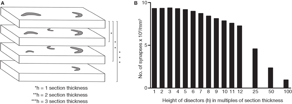
Figure 9. Estimation of the appropriate h value for disectors. In (A), four consecutive sections have been represented and the contours of several synaptic profiles (gray traces) have been drawn. Each disector is calculated on a pair of sections (the reference and look-up sections) separated by a known distance (h). Since the reference and the look-up sections can be swapped to generate another disector, two disectors can be obtained from any pair of sections. If we express h in multiples of the section thickness, it equals 1 for adjacent sections, 2 if we take every second section, and so on. Thus, using four consecutive sections, as in this example, six disectors where h = 1 can be calculated, four disectors where h = 2 and 2 disectors where h = 3. In (B), all possible disectors were calculated on a stack of 114 serial sections. We obtained different estimates of the number of synapses per unit volume for every possible value of h (expressed in multiples of the actual section thickness, 19.9 nm). The graph indicates that values of h up to four times the section thickness (99.5 nm) were acceptable, whereas higher values of h (over about 100 nm) systematically underestimated the number of synapses.
The results obtained by the disector, size-frequency and direct counting methods were similar but not identical (Figure 10
). This is not likely to be due to the fact that the disector and size-frequency methods are usually based on a limited number of samples, since we used all possible disectors within that volume, and all sections were used for the size-frequency method. Thus, theoretically we had the best possible estimate in both cases. The discrepancies are due to the differences in the objects that these methods count. In the direct count, each synapse is a three-dimensional object reconstructed from the traces that appear in several consecutive sections. For example, if we consider the section adjacent to the exclusion plane near the end of a stack, it will most probably contain several synaptic profiles belonging to synaptic junctions that intersect the exclusion plane, and that will therefore not be counted in the direct quantification of synapses. However, the same profiles may be included if we use the disector or the size-frequency methods. In other words, a synaptic junction that intersects any of the exclusion planes in just one section will be excluded from the direct count of objects, whereas the traces of the same synapse that appear in other sections and that do not intersect the exclusion boundary, will be included in the disector and size-frequency methods.
In addition, both the disector and the size-frequency methods are usually applied on a relatively small number of sections (see DeFelipe et al., 1999
), rather than using all the available sections as in the present work. We simulated the results that would have been obtained if limited samples were taken from section stacks (Figure 11
). For example, we ran 10 trials in which 10 pairs of disectors were chosen randomly, 10 trials in which 20 pairs of disectors were chosen randomly, and so on until all possible combinations of disectors were tested. Similarly, we ran a series of trials in which different numbers of sections were selected randomly for the size-frequency method. As expected, the dispersion of the results was highest when fewer sections were selected (Figure 11
). As the numbers of sections considered progressively increased the variability fell, although it never reached zero, even when all possible disectors or sections were accounted for. This is due to the fact that both methods are based on multiple estimates, in contrast to the single estimate obtained from the direct quantification method.
The size-frequency method yields very similar results to the disector method, despite being an assumption-based method. However, it must be pointed out that we have minimized the common errors that occur when using either of these methods with TEM, since both were applied on synapses that had been previously identified and classified through the analysis of serial sections. Specifically, since we used serial sections we strongly diminished the probability of misinterpreting a non-synaptic profile (false synaptic contact) as a truly synaptic contact or vice versa. This is because when using single sections to apply the size-frequency method, or pairs of sections in the case of the disector method, the researcher may not correctly identify synaptic densities. This may occur particularly if the synapses are obliquely cut or en face, or if the synaptic junction is sectioned near one of its borders and thus, the profile appears as only a small dense patch on the microphotograph.
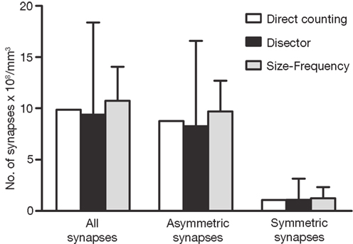
Figure 10. Comparision of the results obtained by directly counting synapses within the counting brick, the disector and the size-frequency methods. The calculation of the number of synapses per unit volume derived by directly counting synaptic junctions within a counting brick of 114 serial sections is represented by white bars. The estimations obtained by means of all possible disectors whose h value was three times the section thickness are shown as black bars (see text and Figure 9
). Grey bars represent the estimations performed by means of the size-frequency method on all sections. All data were calculated on the same stack of sections. Data obtained from the direct count of the synaptic junctions are unique for a single tissue brick, while data obtained by the disector and size-frequency methods are derived from multiple estimations and they are expressed as the mean ± standard deviation. The results of the three methods are similar but not identical. The differences between the means of the disector and size-frequency methods were not statistically significant. Note that the standard deviations were systematically larger for the disector method.
Finally, despite the fact that the size-frequency and the disector methods give similar estimates of the number of synapses, their efficiency was different. From a statistical point of view, efficiency is related to variability: the higher the variability, the lower the efficiency of the method (Baddeley and Vedel Jensen, 2005
). In practice, efficiency is related to the time and effort necessary to obtain a similarly reliable result with both methods. In the present study the disector method was clearly less efficient than the size-frequency method, which means that using a comparable number of samples, the statistical variability of the disector was always higher than that of the size-frequency method (Figures 10 and 11
).
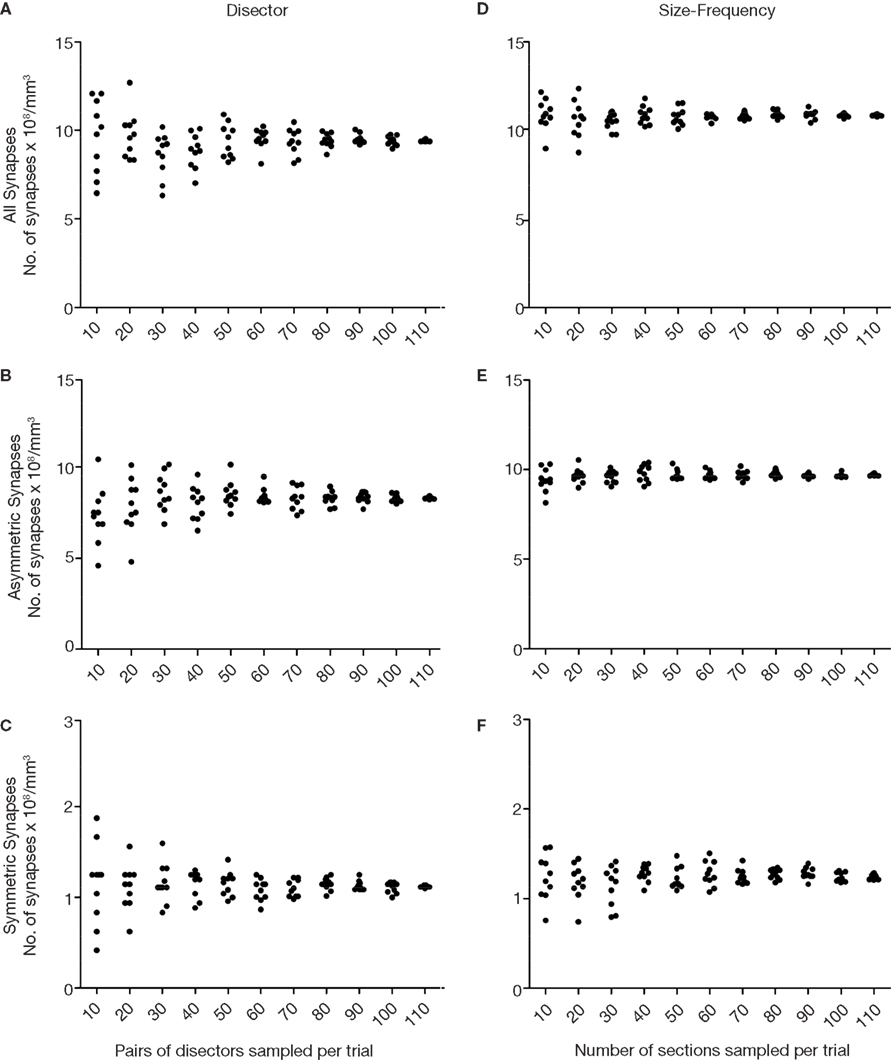
Figure 11. Simulations of the disector and size-frequency methods using different numbers of sections. The data were derived from the same stack of 114 sections used in Figure 10
. In (A), (B) and (C), disectors whose h value was three times the section thickness were used (see text and Figure 9
). The simulation for each type of synapse was carried out as follows. First, 10 pairs of sections were chosen randomly and all the disectors were employed, calculating and plotting the mean value (black dots). This procedure was repeated 10 times. Subsequently, we ran another 10 trials randomly selecting 20 pairs of sections on each trial, and then we ran 10 trials of 30 pairs of sections each, and so on until 10 trials of 110 pairs of sections had been run. As expected, the dispersion of data was less when more pairs of sections were sampled. A similar procedure was followed for the size-frequency method shown in (D), (E) and (F), although single sections instead of pairs of sections were used in each trial. The dispersion of the data also tended to reduce as the number of sections sampled in each trial increased. Note that the size-frequency method showed a smaller dispersion of data than the disector. Calculations for all, asymmetric and symmetric synapses were run independently.
Numerous studies have tried to find simple and accurate methods to estimate the distribution, size and number of synapses. As such, several methods are currently available even though most are based on sampling relatively few single sections. However, serial-section reconstruction should be the method of choice when the final goal is to understand three-dimensional characteristics, such as the number of synapses per unit volume, or location, size and shape of synapses. Indeed, serial sectioning TEM is a well established and mature technique to obtain 3D data from ultrathin sections of brain tissue (Stevens et al., 1980
; Harris et al., 2006
; Hoffpauir et al., 2007
; Kubota et al., 2009
). This method is based on imaging ribbons of consecutive sections with a conventional TEM. Indeed, this approach has often been successfully applied to study the three-dimensional structure of relatively small portions of neurons such as dendritic segments, dendritic spines, axon initial segments or axon terminals (e.g., Porter and White, 1986
; White, 1989
; Fariñas, and DeFelipe, 1991
; Harris, 1999
; Merchán-Pérez et al., 2009
). Extensive reconstructions of single neurons (e.g., White and Rock, 1980
; Megías et al., 2001
) or full reconstructions of small nervous systems or synaptic circuits (Fahrenbach, 1985
; White et al., 1986
) have also been performed, although for technical reasons these studies are rather scarce. The major limitation is that obtaining long series of ultrathin sections is extremely time-consuming and difficult, often making it impossible to reconstruct large volumes of tissue. This is due to the fact that some important problems must be overcome, including the loss of sections, uneven section thickness, the frequent presence of debris or artifacts in sections (e.g. folds) and geometrical distortions. Resolving these problems generally requires labor-intensive human interaction and training, which impairs these approaches from being widely used.
As a result, most studies are currently based on the analysis of a limited sample of single sections, as well as on the application of stereological methods that allow us to deduce the three-dimensional characteristics of synaptic junctions observed in two-dimensions, and to estimate their size and number in a given volume of tissue. The theoretical background of these stereological methods and the formulae to estimate the numbers of synapses per unit volume of cortical tissue has been dealt with in numerous studies (e.g., Mayhew, 1979
, 1996
; Sterio, 1984
; Gundersen et al., 1988a
,b
; Royet, 1991
; Coggeshall and Lekan, 1996
; Mayhew and Gundersen, 1996
; Witgen et al., 2006
). The size-frequency method is an assumption-based method because it assumes that synaptic membrane densities form a polydispersed population of disk-shaped particles (Colonnier and Beaulieu, 1985
). On the other hand, the disector method is considered to be unbiased because it does not depend on the size or shape of synaptic profiles, and it has been claimed to be more reliable than other methods. Thus, the disector has been recommended as the method of choice by numerous authors (Coggeshall and Lekan, 1996
; Mayhew, 1996
; see also Geinisman et al., 1996
), although its results are comparable to those obtained with the size-frequency method (DeFelipe et al., 1999
). In our study, both the disector and the size frequency methods gave similar results to the direct counting of synapses when all the sections available were used. However, in practice fewer sections are used (see DeFelipe et al., 1999
), increasing the statistical variability and lowering the reliability of these methods with respect to the direct counting of synapses. Furthermore, in most methodological studies synapses are simply considered as test objects, without considering that a variety of morphological types of synapses exist in the brain and their functional significance. Indeed, some types of synapses are relatively scarce, whereas others are very numerous. While stereological approaches may be useful to estimate the total number of synapses, they are limited in estimating the proportion of asymmetric (excitatory) and symmetric (inhibitory) synapses, since around 40–60% of the synaptic profiles cannot be characterized from the analysis of single sections (reviewed in DeFelipe et al., 1999
, 2002
). This is because the synaptic cleft and the pre- and post-synaptic densities are often blurred if the section is not at right angles to the synaptic junction, the most extreme case being the en face view, when the plane of section is parallel to the plane of the synaptic junction (see Peters and Kaiserman-Abramof, 1969
). For this reason, uncharacterized synapses are included in the counts as asymmetric and symmetric types, according to the relative frequency of both types of synapse already estimated (DeFelipe et al., 1999
). Although this would seem to be suitable to obtain a good estimate of the proportion of these two types of synapses per unit volume, it is not possible to define their precise spatial distribution. In addition, to estimate the size of large numbers of synapses, the most common method is to measure the cross-sectional lengths of synaptic junctions (synaptic apposition length) to obtain the mean values of the asymmetric and symmetric synapses in a given region. Thus, the size of the synaptic contacts estimated with these methods gives only a rough approximation of the actual size of the post-synaptic areas of the synapses. Furthermore, a significant number of synapses are not identified in single sections, especially when the plane of section is parallel or at a slight angle to the synaptic cleft. This issue has been dealt with by Kubota et al. (2009)
, who concluded that about one-third of synapses on dendritic shafts would not be identified, causing an underestimation in the counts obtained by traditional methods. All these problems can be solved with the use of serial sections and three-dimensional reconstructions, where all synapses can be classified as asymmetric or symmetric (since an uncharacterized synapse in any given section can normally be identified as asymmetric or symmetric in other sections of the series) and the area of the post-synaptic density can be accurately measured.
FIB/SEM microscopy also offers the advantage that the process of obtaining serial images is fully automated, eliminating the need for serial sectioning, the collection of ultrathin sections and the manual acquisition of microphotographs. Moreover, given that the images are taken from the block face, they are almost completely aligned, and the completion of alignment can be fully automated. The resolution that can be obtained in the x–y plane is comparable to that of TEM, since resolutions of around 4 nm/pixel are easily attained. Moreover, the resolution in the z-axis, in our case approximately 20 nm, is even better than that of TEM, where uniform serial sections below 50 nm are extremely difficult to obtain. This new technology is also free of most of the main artifacts of TEM such as the loss or folding of sections, while other problems are reduced to a minimum, like section deformation. The main disadvantage is that each section is destroyed to mill the next one, so it is impossible to study it again if the original images did not give the appropriate information at the working resolution. Hence, visualizing a given object in greater detail in a FIB/SEM image is limited by the resolution of the stack of images. However, this can be compensated by the fact that a single 150 μm thick vibratome section (such as those used in this study) can be sampled in many different locations and under different settings if needed. By contrast, for TEM the vibratome sections have to be trimmed to a relatively small block, loosing a large portion of the material.
In summary, three-dimensional reconstructions are very important to study synaptic connectivity and function, and they help unravel the extraordinary complexity of the nervous system (DeFelipe, 2009
). Indeed, one of the principal goals in neuroscience is to define the microcircuits that exist in the brain and how they contribute to its functional organization, both in health and disease. In this regard, the combination of FIB/SEM microscopy with other techniques, such as those used for physiological characterization of intracellularly-labeled neurons or to retrogradely label neurons projecting to particular brain areas, will greatly help map and examine the afferent and efferent connections of such labeled cells. In turn, as more detailed synaptic circuit diagrams become available, we will learn more about the role of each element in the circuit through computer simulations. Ultimately, this information should enable us to correlate the responses of individual neurons with the activity of microcircuits, an attractive bridge between anatomy, physiology and computation (Segev and London, 2000
; Markram, 2006
). Full reconstruction of whole brains or particular circuits at the electron microscope level is possible in some invertebrates. Indeed, it has been achieved for the relatively small nervous system of the nematode Caenorhabditis elegans (White et al., 1986
). However, even for a small mammal like the mouse, it is impossible to fully reconstruct the brain at the ultrastructural level. For example, if we were to use sections of about 35 μm2 at a thickness of 20 nm, as used in the present study, we would need over 1.4 × 10⁹ sections to fully reconstruct just 1 mm3 of tissue. Therefore, while reconstruction of small regions of the mammalian brain (in the micrometer scale) is feasible, structures like the cerebral cortex, with a surface area of 2,200 cm2 and a thickness that varies between 1.5 and 4.5 mm in humans, cannot be fully reconstructed. It is important to bear in mind that although the number of synapses within a given area and layer may vary, this variability remains within a relatively narrow window. For example, in the rat hindlimb somatosensory cortex, the number of synaptic profiles per 100 μm2 of neuropil varies between 32 and 46 (DeFelipe et al., 2002
). Similarly, it is expected that the variation among the ultrastructural characteristics will also fall within narrow windows or, at least, the statistical distribution of that variation may be modeled. The estimation of this distribution can be achieved by means of spatial sampling strategies (e.g., Lafratta, 2006
). Therefore, we do not need to reconstruct the whole layer within a given cortical region to define the absolute number and types of synapses, and to study their ultrastructural characteristics, but rather the range of variability can be ascertained by multiple sampling of relatively small volumes within that region. Since large extensions of tissue can be efficiently sampled in three-dimensions by the FIB/SEM microscopy we have tested, this new three-dimensional ultrastructural technology will represent a true revolution in examining the microanatomy of the cerebral cortex and of the nervous system in general, opening up new horizons and opportunities to unravel the complexity of the nervous system.
The authors declare that this research was carried out in the absence of any commercial or financial relationships that could be construed as a potential conflict of interest.
We thank A.I. García, I. Fernaud and D. Jiménez for technical assistance. This work was supported by grants from: CIBERNED, the Spanish Ministerio de Educación, Ciencia e Innovación (BFU2006-13395; SAF2009-09394 and Cajal Blue Brain Project) and the Blue Brain Project (EPFL).
The Supplementary Material for this article can be found online at http://www.frontiersin.org/neuroanatomy/paper/10.3389/neuro.05/018.2009/
Supplemental Legends
Supplemental Video 1 | Video sequence made up of 115 consecutive sections from the thin neuropil. Intermingled neuronal and glial processes can easily be followed in successive serial sections. Intracellular structures such as neurofilaments, vesicles, cisternae and mitochondria can also be visualized. Note, for example, the very long mitochondrion that appears at the center of the image. Numerous synapses can also be identified, most of them asymmetric. Field width, 6.44 micrometers.
Supplemental Video 2 | Higher magnification of the upper right corner of the region shown in Supplemental Video 1. Several asymmetric and symmetric synapses can be identified. Some of these synapses have been shown in Figures 3 and 4. Field width, 3.41 micrometers.
Gundersen, H. J. G., Bagger, P., Bendtsen, T. F., Evans, S. M., Korbo, L., Marcussen, N., Møller, A., Nielsen, K., Nyengaard, J. R., Pakkenberg, B., Sørensen, F. B., Vesterby, A., and West, M. J. (1988a). The new stereological tools: disector, fractionator, nucleator and point sampled intercepts and their use in pathological research and diagnosis. APMIS 96, 857–881.
Gundersen, H. J. G., Bendtsen, T. F., Korbo, L., Marcussen, N., Møller, A., Nielsen, K., Nyengaard, J. R., Pakkenberg, B., Sørensen, F. B., Vesterby, A., and West, M. J. (1988b). Some new, simple and efficient stereological methods and their use in pathological research and diagnosis. APMIS 96, 379–394.