Automated Pulmonary Nodule Detection System in Computed Tomography Images: A Hierarchical Block Classification Approach

Abstract

A computer-aided detection (CAD) system is helpful for radiologists to detect pulmonary nodules at an early stage. In this paper, we propose a novel pulmonary nodule detection method based on hierarchical block classification. The proposed CAD system consists of three steps. In the first step, input computed tomography images are split into three-dimensional block images, and we apply entropy analysis on the block images to select informative blocks. In the second step, the selected block images are segmented and adjusted for detecting nodule candidates. In the last step, we classify the nodule candidate images into nodules and non-nodules. We extract feature vectors of the objects in the selected blocks. Lastly, the support vector machine is applied to classify the extracted feature vectors. Performance of the proposed system is evaluated on the Lung Image Database Consortium database. The proposed method has reduced the false positives in the nodule candidates significantly. It achieved 95.28% sensitivity with only 2.27 false positives per scan.

1. Introduction

The primary cause of cancer-related death is lung cancer [1]. Moreover, the mortality of lung cancer is higher than other cancers. The five-year relative survival rate of lung cancer is only 16%; however, if defective nodules are detected at an early stage, the survival rate can be increased [2]. In lung cancer research, computed tomography (CT) is one of the most sensitive methods for detecting pulmonary nodules, where a nodule is defined as a rounded and irregular opaque figure on a CT scan, with a diameter up to 30 mm. The early detection of pulmonary nodules is important in the treatment of lung cancer. However, a CT scan has a large number of images that must be interpreted by a radiologist, which is a fatiguing process. As such, the use of a computer-aided detection (CAD) system can provide an effective solution by assisting radiologists in increasing the scanning efficiency and potentially improving nodule detection [3,4].

Generally, a nodule detection system consists of three main steps: lung volume extraction, nodule candidate detection, and false positive reduction [4]. There are a variety of methods for extracting lung volume from a pulmonary CT scan. In order to segment lung, approaches such as global thresholding [5,6], optimal thresholding [7,8], three-dimensional (3-D)-adaptive fuzzy thresholding [9], rule-based region growing [10], connected component labeling [11], graph-cut algorithm [12], and hybrid segmentation [13] have generally been used. After initial segmentation, lung volume has been extracted using several methods, and the extracted lung volume needed to be refined to include juxta-pleural nodules. For these purposes, morphological approaches [8,14], a rolling ball algorithm [5,15], and a chain code representation-based method [9] have been presented.

The nodule candidates in the segmented lung volume have been detected and segmented before nodule detection. In the literature, various methods have been proposed for detecting nodule candidates. Multiple gray-level thresholding [5,6,15] is one of the most popular methods. Moreover, template-matching-based methods [7], shape-based methods [9,16], filtering-based methods [8], and morphological approaches with convexity models [17] have been used to detect nodule candidates. In this step, there were many false positives which were reduced through false positive reduction.

For over a decade, several feature extraction methods and nodule detection methods have been proposed to reduce false positives. Usually, the reported CAD systems segmented the detected nodule candidates, and then features were extracted from the segmented nodule candidates. The popular features are geometric feature (volume, sphericity, radius of the equivalent sphere, maximum compactness, maximum circularity, and maximum eccentricity), gray level features (mean gray level with in the segmented object, standard deviation of gray level, and moments of gray level), and gradient features [5,6]. Finally, nodules were detected through various classifiers using the extracted feature vectors with a small amount of false positives. The rule-based filtering method [7] and linear discriminant analysis classifier [5,8] have been generally used. In addition, machine learning-based classification methods have been also used for false positive reduction. These methods are based on genetic algorithm [9], genetic programming [6], neural network [18], and support vector machine [11]. There are many CAD systems for detecting nodules which have different strengths and weaknesses. In order to increase the strength of CAD systems, Niemeijer et al. presented generic methods to combine multiple CAD systems [19].

In this paper, we propose a novel pulmonary nodule detection method based on hierarchical three-dimensional (3-D) block classification. In the following sections, each stage of the proposed CAD system is described in detail. The remainder of the paper is organized as follows. In Section 2, we briefly describe the methods used in this work. Section 3 presents a 3-D block image selection method based on entropy analysis. Section 4 describes a 3-D block analysis to detect nodule candidates. In Section 5, support vector machine (SVM) classifiers are described to detect pulmonary nodules. In Section 6, we discuss the experimental results obtained with the proposed method, and finally, in Section 7, we provide conclusions.

2. Proposed Method

In this paper, a hierarchical 3-D block analysis method is proposed to detect pulmonary nodules on CT images. A block diagram of the proposed CAD system is shown in Figure 1. The proposed CAD system consists of three steps. In the first step, we split input CT images into block images and non-informative blocks are filtered out. In the second step, nodule candidates are detected. We segment objects in the selected block images and adjust their location to detect the nodule candidates. In the last step, we classify the nodule candidates into nodules and non-nodules. Feature vectors are extracted from the object in the nodule candidate blocks. SVM classifiers are applied to the extracted feature vectors to detect nodules. The proposed method provides improved accuracy and reduces the false positive rate. It is evaluated on the Lung Image Database Consortium (LIDC) database [20]. The LIDC is a publicly available database of thoracic CT scans as a medical imaging research resource. The proposed method extremely reduced the false positives in the nodule candidates with high sensitivity.

Figure 1. Flow chart of the proposed nodule detection system.

Figure 1. Flow chart of the proposed nodule detection system.

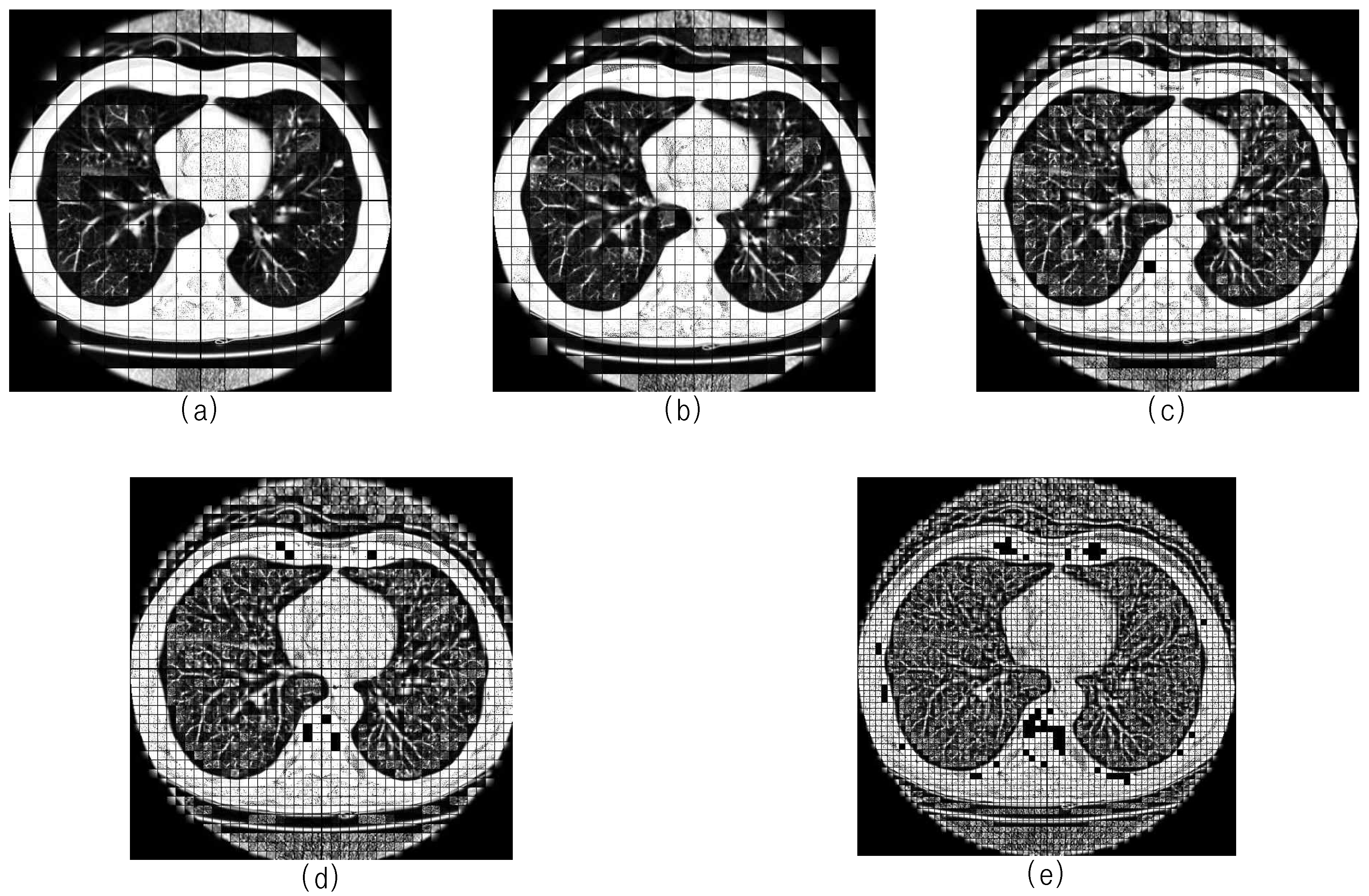
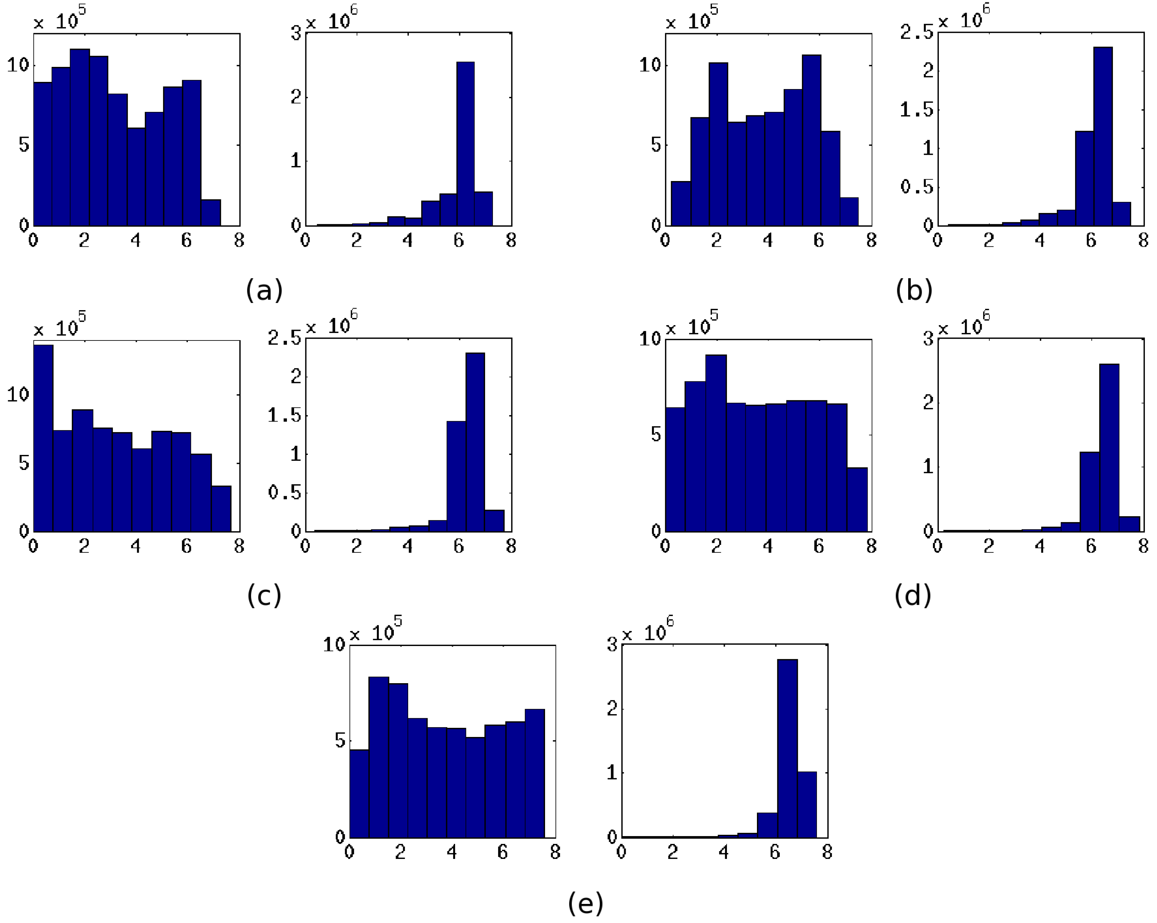
3. Three-Dimensional Block Image Selection Based on Entropy Analysis

In order to analysis block images, we split a 3-D CT scan into 3-D block images, and we filter out the non-informative blocks. Five different sizes (32, 24, 16, 12, and 8) of 3-D block images are applied to detect different sizes of nodules. The split block images are shown in Figure 2. Moreover, this hierarchical multi-scale approach gives advantages of the computational efficiency and robustness. The proposed block analysis is performed hierarchically from rough form to detail, and it is employed in order of decreasing block size. We can detect proper size of nodules in each size of blocks and all the parts of target object should be in the selected block image. For example, the inner part of the big object at the small block image is a uniform region and its entropy is very small. In this case, we do not need to analyze the small block image because the big object can be detected at the larger-sized block image.

Figure 2. Result images after block splitting with respect to various block sizes, (a) 32; (b) 24; (c) 16; (d) 12; and (e) 8.

Figure 2. Result images after block splitting with respect to various block sizes, (a) 32; (b) 24; (c) 16; (d) 12; and (e) 8.

In order to efficiently analyze, we need to filter out non-informative block images. If non-informative blocks are removed from a larger-sized block, we do not need to analyze that area on smaller-sized blocks. For this task, we propose the entropy-based block selection method. In information theory, entropy is a measure of the uncertainty associated with a random variable [21]. We can measure image information content using entropy [22,23]. Therefore, we can classify block images into informative and non-informative categories using image entropy.

First, we calculate entropy values on every block image to select informative blocks. Entropy of block image is calculated by follows:

$$E=-\sum _{i=0}^{n}p\left(i\right)lo{g}_2\left(p\left(i\right)\right)$$

(1)

where $p\left(i\right)$ is the probability of pixel intensity in block image corresponding to intensity i. We can simply select the informative block images using entropy value.

$$\left\{\begin{array}{cc}\left(\mathrm{informative}\right),& if{T}_l\le E\le T_h\\ (\mathrm{non}-\mathrm{informative}),& \mathrm{Otherwise}\end{array}\right..$$

(2)

where $T_l$ is lower threshold and $T_h$ is higher threshold for entropy value. If entropy E is lower than $T_l$, the input block image has no content. On the other hand, if entropy E is higher than $T_h$, the block image is noise.

We select the thresholds of entropy using histogram which is obtained from the informative regions on the selected CT images. The informative regions are defined by using the location of the nodules which are annotated by radiologists. As shown in Figure 3, the informative blocks have the specific entropy values on every block size. The thresholds of entropy selecting the informative blocks are ranged four to eight which can cover almost every informative region. The informative blocks are selected by using the proposed block image selection method based on entropy analysis. These block images will be analyzed for detecting nodules.

Figure 3. The entropy histograms of block images using five different block sizes, left: non-informative blocks, right: informative blocks; (a) 32; (b) 24; (c) 16; (d) 12; and (e) 8.

Figure 3. The entropy histograms of block images using five different block sizes, left: non-informative blocks, right: informative blocks; (a) 32; (b) 24; (c) 16; (d) 12; and (e) 8.

4. Nodule Candidates Selection Based on Block Analysis

The nodule candidate block images are selected in this step. The informative block images are enhanced before segmentation. We segment the objects in the selected block images and adjust the location of block image.

4.1. Block Image Enhancement

We propose the block image enhancement method for more accurate analysis. Several filtering methods have been used for image enhancement. The Gaussian and median filters are general methods for smoothing, however, these filters cannot preserve edge and structure. For edge-preserving filtering, bilateral filters have been used, though the bilateral filter is able to enhance only plate-like structures in 3-D images. We apply 3-D coherence-enhancing diffusion (CED) filter to remove noise in the block image I. 3-D CED filter can preserves small spherical structures and enhance tubular structures. Therefore, 3-D CED is more suitable for pulmonary nodule detection than bilateral filter [24]. The basis for a 3-D CED filter is introduced by Weickert et al. [25].

First of all, we need to calculate the Hessian $\mathbf{H}$ from every pixel of the Gaussian smoothed input image G. The Hessian matrix of 3-D image (eg. medical image (x,y,z)) is represented as follows:

$$\mathbf{H}=\left[\begin{array}{ccc}{G}_{xx}& G_{xy}& G_{xz}\\ G_{xy}& G_{yy}& G_{yz}\\ G_{xz}& G_{yz}& G_{zz}\end{array}\right]$$

(3)

Gaussian image smoothing is performed prior to the calculation of the gradient to reduce the effect of the noise,

$$G(I(x,y,z),\sigma )=\frac{1}{2\pi {\sigma }^2}{e}^{-\frac{x^2+y^2+z^2}{2{\sigma }^2}}$$

(4)

where $I(x,y,z)$ is the input block image and σ is the noise reduction parameter. Next, we calculate eigenvalue decomposition of Hessian $\mathbf{H}$. Image edges give large eigenvalues, and the eigenvectors corresponding to those eigenvalues describe the direction of the edge. The eigenvectors are used as diffusion tensor directions. The amplitude of the diffusion in those three directions is based on the eigenvalues and determined by Weickerts equation [25]. A finite difference scheme is used to do the diffusion. This process is repeated until a certain diffusion time is reached. Figure 4 shows before and after applying the 3-D CED filtering on the input block image. The enhanced block image B will be analyzed to detect nodule candidates in the following section.

Figure 4. (a) Input image and (b) the result image after enhancement.

Figure 4. (a) Input image and (b) the result image after enhancement.

4.2. Block Segmentation and Location Adjustment

To segment object in the enhanced block image B, we applied a optimal thresholding method. In CT scans, air has an attenuation of $-1000$ Hounsfield Units (HU). Nodules are dense objects and their intensity is above $-500$ HU [26]. Therefore, we set $-500$ HU as the initial threshold $T^{\left(0\right)}$ for iteratively computing the threshold to start the iteration. For this task, let $T^{\left(i\right)}$ be the threshold after the $i^{th}$ step; to choose a new threshold, we apply $T^{\left(i\right)}$ to the block image. Let ${\mu }_o$ and ${\mu }_b$ be the mean intensities of the object and background in the block image, respectively, and the new threshold becomes

$$T^{(i+1)}=\frac{{\mu }_o+{\mu }_b}{2}$$

(5)

Note that this iterative approach continues until the threshold converges, and the optimal threshold $T_{op}$ is obtained. As such, an initial segmented block image O can be obtained by thresholding all of the non-object voxels as follows:

$$O(x,y,z)=\left\{\begin{array}{ccc}1& \left(\mathrm{object}\right),& \mathrm{if}\mathit{B}(\mathit{x},\mathit{y},\mathit{z})>{\mathit{T}}_{\mathit{op}}\\ 0& (\mathrm{non}-\mathrm{object}),& \mathrm{Otherwise}\end{array}\right.$$

(6)

After segmentation, we adjust the location of the block because the segmented object is not located in the center of the block image. The block location is iteratively updated by using the centroid of the segmented object O. The iteration of the adjustment continues until the center position of the block image converges, and the distance between the adjusted location and the original location of the block image is larger than half of the block size. In this case, the object in the block image is a part of the vessel, or is too big. The iterations of block location adjustment are shown in Figure 5. Nodule candidate block images are selected after iterative adjustment of block location.

Figure 5. Iterations of automatic block location adjustment, upper: 3-D shapes, lower: the median slices of 3-D block; (a) the first; (b) the fifth; and (c) the last iterations of adjustment.

Figure 5. Iterations of automatic block location adjustment, upper: 3-D shapes, lower: the median slices of 3-D block; (a) the first; (b) the fifth; and (c) the last iterations of adjustment.

5. Nodule Detection

In order to detect the nodules, we extract feature vectors from the detected nodule candidates. Next, the feature vectors become the input for classifier and classified into nodules and non-nodules.

5.1. Feature Extraction

The nodule candidate block images are selected from the previous step. We extract three different types of features from a nodule candidate block image $I_{NC}$, namely, 2-D geometric, 3-D geometric, and 2-D texture features. Moreover, in the literature, a similar type of feature has been extracted by different researchers for this application [5,15]. The 2-D features are extracted from a median slice $I_{NC,m}$ of nodule candidates because the area of the segmented object at the median slice is the largest.

Nodules have their own shapes which are important characteristics for distinguishing from the other objects in lung. 2-D and 3-D geometric features describe the shapes of the nodule candidates. The 2-D geometric features consist of an area ($x_1$), diameter ($x_2$) and circularity ($x_3$), which are based on cross-sectional images of nodule candidates. The area is obtained as follows:

$$A=\sum _{o\in O_m}o$$

(7)

where $O_m$ is a median slice of the segmented object O. Diameter D is a maximum bounding box length of $O_m$. The circularity is computed by dividing the area by the squared perimeter of the circumscribed circle as follows:

$$Circ=\frac{A}{4\pi r^2}$$

(8)

where r is the radius of the circumscribed circle and it is equal to $\frac{D}{2}$. 3-D geometric features comprise the volume ($x_4$), compactness ($x_5$), and elongation ($x_6$). The volume of the segmented object O is computed as:

$$Vol=\sum _{o\in O}o$$

(9)

and compactness is calculated as follows:

$$Cmp=\frac{Vol}{\frac{4}{3}\pi r^3}$$

(10)

Elongation is the ratio between the first principal axis length $PA{L}_1$ and the second principal axis length $PA{L}_2$ as follows:

$$El=\frac{PA{L}_1}{PA{L}_2}$$

(11)

where the three principal axis lengths are the lengths of all of the principal axes of the segmented object volume O.

In order to increase accuracy of classification, we also use 2-D texture features which consist of mean ($x_7$), variance ($x_8$), skewness ($x_9$) and kurtosis ($x_{10}$) of the median slice $I_{NC,m}$ of the nodule candidates block image $I_{NC}$. Moreover, the eight largest eigenvalues ($x_{11}\sim x_{18}$) of $I_{NC,m}$ are obtained. Mean (μ), variance (${\sigma }^2$), skewness (${\gamma }_1$) and kurtosis (${\gamma }_2$) are calculated as follows:

$$\mu =\frac{1}{N}\sum _{i\in I_{NC,m}}i$$

(12)

$${\sigma }^2=\frac{1}{N}\sum _{i\in I_{NC,m}}{(i-\mu )}^2$$

(13)

$${\gamma }_1=\frac{1}{N}\sum _{i\in I_{NC,m}}{\left(\frac{i-\mu }{\sigma }\right)}^3$$

(14)

and

$${\gamma }_2=\frac{1}{N}\sum _{i\in I_{NC,m}}{\left(\frac{i-\mu }{\sigma }\right)}^4-3$$

(15)

where N is the number of pixels in $I_{NC,m}$.

In this way, we extract 18 features $\mathbf{x}=\{x_1,...,x_{18}\}$ from the nodule candidates. The summary of the extracted features is shown in Table 1. The feature vector $\mathbf{x}$ is provided as the input vector for the training of the classifier.

Table 1. Feature list for nodule detection.

Index	Feature	Description
2-D geometric feature vectors
$x_1$	Area	Number of pixels in the median slice $O_m$ of the segmented object O
$x_2$	Diameter	Maximum bounding box length of $O_m$
$x_3$	Circularity	Area $x_1$ divided by squared perimeter of the circumscribed circle $4\pi r^2$ where $r=\frac{x_2}{2}$
3-D geometric feature vectors
$x_4$	Volume	Total count of voxels in the segmented object O
$x_5$	Compactness	Volume $x_4$ divided by volume of the circumscribed sphere $\frac{4}{3}\pi r^3$
$x_6$	Elongation	Ratio between maximum principal axis length and minimum principal axis length
2-D texture feature vectors
$x_7$	Mean	Mean intensity of the median slice $I_{NC,m}$ of nodule candidates block image $I_{NC}$
$x_8$	Variance	Variance intensity of $I_{NC,m}$
$x_9$	Skewness	Skewness intensity of $I_{NC,m}$
$x_{10}$	Kurtosis	Kurtosis intensity of $I_{NC,m}$
$x_{11}\sim x_{18}$	Eigenvalues	Eight largest eigenvalues of $I_{NC,m}$

Table 1. Feature list for nodule detection.

Index	Feature	Description
2-D geometric feature vectors
$x_1$	Area	Number of pixels in the median slice $O_m$ of the segmented object O
$x_2$	Diameter	Maximum bounding box length of $O_m$
$x_3$	Circularity	Area $x_1$ divided by squared perimeter of the circumscribed circle $4\pi r^2$ where $r=\frac{x_2}{2}$
3-D geometric feature vectors
$x_4$	Volume	Total count of voxels in the segmented object O
$x_5$	Compactness	Volume $x_4$ divided by volume of the circumscribed sphere $\frac{4}{3}\pi r^3$
$x_6$	Elongation	Ratio between maximum principal axis length and minimum principal axis length
2-D texture feature vectors
$x_7$	Mean	Mean intensity of the median slice $I_{NC,m}$ of nodule candidates block image $I_{NC}$
$x_8$	Variance	Variance intensity of $I_{NC,m}$
$x_9$	Skewness	Skewness intensity of $I_{NC,m}$
$x_{10}$	Kurtosis	Kurtosis intensity of $I_{NC,m}$
$x_{11}\sim x_{18}$	Eigenvalues	Eight largest eigenvalues of $I_{NC,m}$

5.2. Support Vector Machine Classifier

In order to detect the nodule and to reduce false positives, the feature vector is analyzed by a classifier. SVMs are a useful technique for data classification [27]. In addition, SVMs are supervised learning models with associated learning algorithms that analyze data and recognize patterns, used for classification and regression analysis. The basic SVM takes a set of input data and predicts two possible classes for each given input.

5.2.1. Classifier Training

For training the SVM, the first step is to construct a training dataset comprised of the feature vectors. In this study, the feature vector $\mathbf{x}$ is extracted and selected as explained in Section 5.1. Typically, the number of non-nodules is larger than the number of nodules in nodule candidates. This unbalance in the amount of data may affect the training of the classifier. Therefore, we need to select a balanced number of nodules and non-nodules. To balance the dataset, we randomly select $K/2$ nodules and $K/2$ non-nodules from nodule candidates. The balanced dataset is then randomly split into training and testing datasets in validation of the classifier. The training dataset, $\mathbf{X}={\left\{({\mathbf{x}}_i,y_i)\right\}}_{i=1}^N$, is constructed by selecting N nodule candidates, with each training data pair consisting of an input feature vector and its corresponding known target class. The SVM requires the solution of the following optimization problem:

$$\underset{\mathbf{w},\xi ,b}{min}\left\{\frac{1}{2}{\mathbf{w}}^T\mathbf{w}+C\sum _{i=1}^n{\xi }_i\right\}$$

(16)

subject to (for any $i=1,\dots N$)

$$f\left({\mathbf{x}}_i\right)=y_i({\mathbf{w}}^T\varphi \left({\mathbf{x}}_i\right)-b)\ge 1-{\xi }_i$$

(17)

where ${\xi }_i\ge 0$ and $f\left({\mathbf{x}}_i\right)$ is the decision function. Here, training vectors ${\mathbf{x}}_i$ are mapped into a higher dimensional space by the function ϕ. SVM finds a linear separating hyper plane ($\mathbf{w},b$) with the maximal margin in this higher dimensional space. $C>0$ is the penalty parameter of the error term.

Furthermore, SVMs can efficiently perform non-linear classification using what is called the kernel trick, implicitly mapping their inputs into high-dimensional feature spaces. $K({\mathbf{x}}_i,{\mathbf{x}}_j)\equiv \varphi {\left({\mathbf{x}}_{\mathbf{i}}\right)}^T\varphi \left({\mathbf{x}}_{\mathbf{j}}\right)$ is called the kernel function. In this paper, we use radial basis function $K_r({\mathbf{x}}_i,{\mathbf{x}}_j)$, polynomial function $K_p({\mathbf{x}}_i,{\mathbf{x}}_j)$, and Minkowski distance function $K_m({\mathbf{x}}_i,{\mathbf{x}}_j)$ as kernel functions. The mathematical descriptions of these kernel functions are as follows:

$$K_r({\mathbf{x}}_i,{\mathbf{x}}_j)=exp(\frac{-{∥{\mathbf{x}}_i-{\mathbf{x}}_j∥}^2}{p^2})$$

(18)

$$K_p({\mathbf{x}}_i,{\mathbf{x}}_j)={∥{\mathbf{x}}_i·{\mathbf{x}}_j+1∥}^p$$

(19)

and

$$K_m({\mathbf{x}}_i,{\mathbf{x}}_j)={\left(\sum _{k=1}^M{∥{\mathbf{x}}_{i,k}-{\mathbf{x}}_{j,k}∥}^p\right)}^{\frac{1}{p}}$$

(20)

where $p>0$ and ${\mathbf{x}}_{i,k}$ is the $k^{th}$ element of feature vector ${\mathbf{x}}_i$.

For a SVM training, the non-linear separating hyper plane with the maximal margin in this higher dimensional space is automatically adapted by using the kernel trick. In this manner, the solution space is refined and converges to the optimal/near optimal solution. The training is stopped if the optimized maximal margin hyper plane is obtained for all input training vectors.

5.2.2. Nodule Detection and Classifier Validation

Nodules and non-nodules can be classified effectively by the trained classifier. To obtain the class predicted from the testing data, we need to provide an input feature vector for each nodule candidate. It is important to note that the input data is now different from the training data. The testing data consists of only the input feature vectors, and the target values are unknown. In this case, the trained classifier will predict a class by only taking into account the input feature vectors. The input feature vector $\mathbf{x}$ is obtained as described in Section 5.1. In brief, the lexicographically arranged input feature vectors are first represented in a matrix $\mathbf{X}={\left\{{\mathbf{x}}_{\left(n\right)}\right\}}_{n=1}^N$ of size $N\times M$, where $\mathbf{x}$ represents an M-dimensional feature vector, and N indicates the total number of feature vectors. SVM finds the maximal margin hyper plane in the higher dimensional space of input feature vector in training process. The nodules are then separated from non-nodules by the maximal margin hyper plane in the feature space.

In this paper, we apply k-fold cross-validation to evaluate the proposed classifier. The original sample is randomly partitioned into k equal size sub-samples in k-fold cross-validation. Of the k sub-samples, a single sub-sample is selected as the validation data for testing the model. The remaining $k-1$ sub-samples are used as training data. The cross-validation process is then repeated k times (the folds), with each of the k sub-samples. The k results from the folds are then averaged to produce a single estimation. The advantage of this method over repeated random sub-sampling is that all observations are used for both training and validation, and each observation is used for validation exactly once.

The performance of a classifier could be estimated in terms of the number of true positives and false positives. The performance validation measures are accuracy, sensitivity, specificity, negative predictive value (NPV), Matthews correlation coefficient (MCC) and area under the receiver operating characteristic (ROC) curve. When the graph between the sensitivity and false positive rate is plotted for different threshold values, the resultant curve is called the ROC curve. The ROC curve summarizes how well a classifier performs under different operating conditions for a particular problem. As such, the area under the ROC curve (AUC) is a common index that summarizes the information contained in the curve.

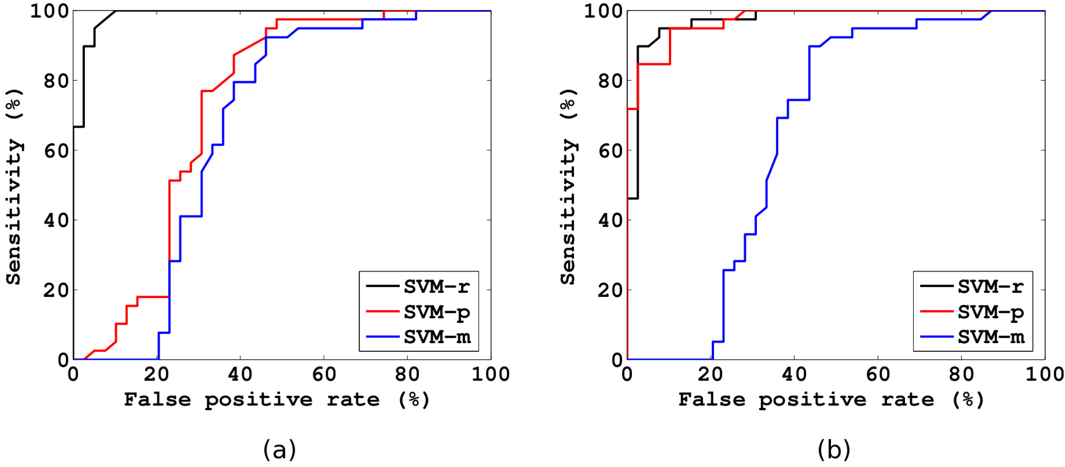
6. Experimental Results and Discussion

Performance of the proposed CAD system is evaluated using the LIDC database [20]. It is publicly available in the National Biomedical Imaging Archive (NBIA), and its nodules have been fully annotated by multiple radiologists. Four expert chest radiologists drew outlines for the nodules with effective sizes of 3 mm or greater. The ground truth has been established by a blinded reading and a subsequent unblinded reading. The LIDC database consists of 84 CT scans, but only 58 CT scans contain nodules. We used 58 CT scans to evaluate the proposed system. All of the annotated nodule segmentations are used in the evaluation of the proposed method. The overlapped manual nodule segmentations from four different radiologists are merged to a single segmentation. This dataset consists of 151 nodules and 10,531 slices. The diameters of the nodules range from 3 to 30 mm. The number of slices per scan is about 200, and each slice has 512 × 512 pixels and 4096 gray level values in HU. The pixel size in the database ranges from 0.5 to 0.76 mm, and the reconstruction interval ranges from 1 to 3 mm.

The nodule candidates are considered as nodules or non-nodules using annotation provided by chest radiologists. In the evaluation, each detected nodule candidate is determined to be a nodule if its distance to any nodule in the database is smaller than 1.5 times the radius of that nodule or if its radius is greater than 0.8 times or smaller than 1.5 times the radius of the target nodule. We denote this classification as a hit. We allow a ”near hit” by using these 0.8 and 1.5 factors, which were obtained by experiments. If a hit on a detected nodule candidate is produced, it will be counted as a true positive. However, if no hit is produced, it will be considered to be a false positive.

The input CT images were divided into block images, and we filtered out the non-informative blocks by using entropy analysis. Next, the nodule candidates were detected from the selected informative block images by using proposed block segmentation method. We segmented the objects in the selected block images and adjust the locations of the blocks. We detected 147 nodules and 3492 non-nodules (false positives) as nodule candidates; sensitivity is 97.35% with 60.21 false positives per scan.

In the last step, we classified the nodule candidates into nodules and non-nodules. We extracted the feature vector of the object in the nodule candidate block images. SVMs were applied to the extracted feature vectors to detect nodules. The proposed SVMs were evaluated by k-fold cross validation where 5, 7, or 10 is typically used as a k. In this paper, 7-fold cross validation is used for evaluation because it provides a more suitable balance between training and testing data for evaluating the proposed method than 5-fold and 10-fold cross validation. Table 2 shows the performance of SVMs for different k values. As shown in Table 2, 7-fold cross validation shows the best results, and there are small differences of performance measures with respect to different k values.

Table 2. The k-fold cross validation results of SVM classifiers with radial basis function kernel for different k values.

k	p	AUC	MCC	NPV	Accuracy	Sensitivity	Specificity
5	0.25	0.9738	0.8312	88.20%	91.52%	87.16%	95.88%
7	0.25	0.9784	0.8816	91.61%	93.97%	91.02%	96.92%
10	0.25	0.9736	0.8548	90.16%	92.43%	88.97%	95.88%

Table 2. The k-fold cross validation results of SVM classifiers with radial basis function kernel for different k values.

k	p	AUC	MCC	NPV	Accuracy	Sensitivity	Specificity
5	0.25	0.9738	0.8312	88.20%	91.52%	87.16%	95.88%
7	0.25	0.9784	0.8816	91.61%	93.97%	91.02%	96.92%
10	0.25	0.9736	0.8548	90.16%	92.43%	88.97%	95.88%

Table 3 shows the performance of SVMs using different kernel functions, SVM-r: radial basis function, SVM-p: polynomial function, and SVM-m: Minkowski distance function. Figure 6 shows the ROC curves of the SVM classifiers with respect to three different kernel functions ((a) $p=0.25$ and (b) $p=1$). The SVM-r shows more accurate and robust results with various kernel parameters. The SVM-p shows quite accurate results when parameter p is $0.5\sim 2$, whereas it is not stable. The performance of classification is generally not strong on the SVM-m.

Table 3. The 7-fold cross validation results of SVM classifiers with three diffrent kernel functions, SVM-r: radial basis function, SVM-p: polynomial function, and SVM-m: Minkowski distance function.

	p	AUC	MCC	NPV	Accuracy	Sensitivity	Specificity
SVM-r	0.1	0.9727	0.7322	76.96%	84.72%	69.44%	100.00%
	0.125	0.9746	0.7990	82.65%	88.96%	78.70%	99.23%
	0.25	0.9784	0.8816	91.61%	93.97%	91.02%	96.92%
	0.5	0.9754	0.8545	91.77%	92.82%	91.54%	94.10%
	1	0.9712	0.8364	91.63%	91.79%	91.53%	92.05%
	2	0.9673	0.8443	93.01%	92.30%	93.08%	91.53%
SVM-p	0.1	0.4660	-0.1486	16.14%	47.40%	0.00%	94.81%
	0.125	0.4632	-0.1095	17.07%	44.81%	0.26%	89.35%
	0.25	0.6876	0.4019	81.78%	68.26%	86.13%	50.39%
	0.5	0.9462	0.8058	92.02%	89.85%	91.52%	88.18%
	1	0.9463	0.8188	92.77%	90.74%	92.78%	88.69%
	2	0.9646	0.8514	92.17%	92.29%	91.25%	93.32%
SVM-m	0.1	0.8706	0.6524	85.72%	82.55%	86.91%	78.19%
	0.125	0.7051	0.4154	75.49%	69.71%	78.46%	60.95%
	0.25	0.5706	0.2300	64.25%	60.68%	68.69%	52.68%
	0.5	0.5469	0.1911	62.02%	59.02%	66.63%	51.41%
	1	0.5420	0.1749	60.93%	58.11%	66.11%	50.12%
	2	0.5527	0.1673	60.56%	57.60%	65.85%	49.36%

Table 3. The 7-fold cross validation results of SVM classifiers with three diffrent kernel functions, SVM-r: radial basis function, SVM-p: polynomial function, and SVM-m: Minkowski distance function.

	p	AUC	MCC	NPV	Accuracy	Sensitivity	Specificity
SVM-r	0.1	0.9727	0.7322	76.96%	84.72%	69.44%	100.00%
	0.125	0.9746	0.7990	82.65%	88.96%	78.70%	99.23%
	0.25	0.9784	0.8816	91.61%	93.97%	91.02%	96.92%
	0.5	0.9754	0.8545	91.77%	92.82%	91.54%	94.10%
	1	0.9712	0.8364	91.63%	91.79%	91.53%	92.05%
	2	0.9673	0.8443	93.01%	92.30%	93.08%	91.53%
SVM-p	0.1	0.4660	-0.1486	16.14%	47.40%	0.00%	94.81%
	0.125	0.4632	-0.1095	17.07%	44.81%	0.26%	89.35%
	0.25	0.6876	0.4019	81.78%	68.26%	86.13%	50.39%
	0.5	0.9462	0.8058	92.02%	89.85%	91.52%	88.18%
	1	0.9463	0.8188	92.77%	90.74%	92.78%	88.69%
	2	0.9646	0.8514	92.17%	92.29%	91.25%	93.32%
SVM-m	0.1	0.8706	0.6524	85.72%	82.55%	86.91%	78.19%
	0.125	0.7051	0.4154	75.49%	69.71%	78.46%	60.95%
	0.25	0.5706	0.2300	64.25%	60.68%	68.69%	52.68%
	0.5	0.5469	0.1911	62.02%	59.02%	66.63%	51.41%
	1	0.5420	0.1749	60.93%	58.11%	66.11%	50.12%
	2	0.5527	0.1673	60.56%	57.60%	65.85%	49.36%

Figure 6. ROC curves of the SVM classifiers with respect to three different kernel functions, SVM-r: radial basis function, SVM-p: polynomial function, and SVM-m: Minkowski distance function; (a) $p=0.25$ and (b) $p=1$.

Figure 6. ROC curves of the SVM classifiers with respect to three different kernel functions, SVM-r: radial basis function, SVM-p: polynomial function, and SVM-m: Minkowski distance function; (a) $p=0.25$ and (b) $p=1$.

Table 4. The overall performance of CAD system for different parameters p of SVM-r classifiers.

p	AUC	MCC	NPV	Accuracy	Specificity	Sensitivity	false positives/scan
Nodule Candidates Detection						97.35%	60.21
0.1	0.9931	0.9594	99.11%	95.89%	99.62%	92.67%	0.23
0.125	0.9934	0.9509	99.35%	96.92%	99.11%	93.95%	0.54
0.25	0.9929	0.8785	99.59%	97.61%	96.23%	95.28%	2.27
0.5	0.9835	0.8082	99.10%	95.15%	93.93%	92.85%	3.65
1	0.9727	0.7602	98.66%	92.98%	92.33%	90.63%	4.62
2	0.9584	0.7101	98.58%	92.41%	89.74%	90.45%	6.18

Table 4. The overall performance of CAD system for different parameters p of SVM-r classifiers.

p	AUC	MCC	NPV	Accuracy	Specificity	Sensitivity	false positives/scan
Nodule Candidates Detection						97.35%	60.21
0.1	0.9931	0.9594	99.11%	95.89%	99.62%	92.67%	0.23
0.125	0.9934	0.9509	99.35%	96.92%	99.11%	93.95%	0.54
0.25	0.9929	0.8785	99.59%	97.61%	96.23%	95.28%	2.27
0.5	0.9835	0.8082	99.10%	95.15%	93.93%	92.85%	3.65
1	0.9727	0.7602	98.66%	92.98%	92.33%	90.63%	4.62
2	0.9584	0.7101	98.58%	92.41%	89.74%	90.45%	6.18

Figure 7. FROC curves of the proposed CAD system with respect to three different kernel parameters of SVM-r classifiers.

Figure 7. FROC curves of the proposed CAD system with respect to three different kernel parameters of SVM-r classifiers.

The overall system performance was then evaluated for all detected nodule candidates. The false positives, which remained after nodule candidate detection, were extremely reduced after applying SVM classification. The overall performance of the proposed CAD system is shown in Table 4. We multiplied sensitivity of SVM classifier by sensitivity of nodule candidate detection to obtain the overall sensitivity of the proposed CAD system. The proposed method shows excellent classification results. Accuracies of classification are more than 90% and their sensitivities are also over 90%. The best accuracy is 97.61% when the parameter p is $0.25$. In Figure 7, the overall performance of the proposed CAD system is represented by the free-response ROC (FROC) curves. The proposed methods show robust and accurate performance in detecting nodules.

It is difficult to compare previously published CAD systems due to different datasets, nodule types, sizes, and validation methods. However, it is important to compare the performance of the proposed system. We selected recently reported CAD systems to compare their performances. Half of them used the LIDC database [5,6,28]. The other half of the papers used their own databases. Table 5 shows the comparison of the proposed CAD system with previously reported CAD systems. The different CAD systems have shown reasonable sensitivity values in pulmonary nodule detection. Our proposed method shows significantly high sensitivity with reduced false positives.

Table 5. Performance comparison of reported CAD system.

CAD systems	Nodule size	Sensitivity	Avg. false positives /scan
Dehmeshki et al.(2007) [7]	3-20 $mm$	90%	14.6
SuarezCuenca et al.(2009) [8]	4-27 $mm$	80%	7.7
Opfer and Wiemeker(2007)[28]	≥4 $mm$	74%	4
Messay et al.(2010) [5]	3-30 $mm$	82.66%	3
Choi et al.(2012) [6]	3-30$mm$	94.1%	5.45
Proposed method	3-30 $mm$	95.28%	2.27

Table 5. Performance comparison of reported CAD system.

CAD systems	Nodule size	Sensitivity	Avg. false positives /scan
Dehmeshki et al.(2007) [7]	3-20 $mm$	90%	14.6
SuarezCuenca et al.(2009) [8]	4-27 $mm$	80%	7.7
Opfer and Wiemeker(2007)[28]	≥4 $mm$	74%	4
Messay et al.(2010) [5]	3-30 $mm$	82.66%	3
Choi et al.(2012) [6]	3-30$mm$	94.1%	5.45
Proposed method	3-30 $mm$	95.28%	2.27

7. Conclusions

In order to detect defective nodules, we have proposed a novel CAD system based on hierarchical 3-D block image analysis. Firstly, we hierarchically split the input CT images into 3-D block images, and the block images were classified into informative and non-informative by using the entropy analysis. Next, the selected informative block images were analyzed to detect nodule candidates. Finally, we detected nodules from the detected nodule candidates using the proposed classification method. We extracted feature vectors from the detected nodule candidates, and the feature vectors were classified into nodule and non-nodule by using the SVM classifier. The performance of the proposed system was evaluated on the LIDC database. The proposed method has reduced the false positives in nodule candidates significantly. It achieved 95.28% sensitivity with only 2.27 false positives per scan and its accuracy was 97.61%. The results have shown the superiority of the proposed method.

References

1. Jemal, A.; Siegel, R.; Ward, E.; Hao, Y.; Xu, J.; Thun, M.J. Cancer statistics, 2009. CA: Cancer J. Clin. 2009, 59, 225–249. [Google Scholar] [CrossRef] [PubMed]
2. Bach, P.; Mirkin, J.; Oliver, T.; Azzoli, C.; Berry, D.; Brawley, O.; Byers, T.; Colditz, G.; Gould, M.; Jett, J.; et al. Benefits and harms of CT screening for lung cancer. Context 2012, 307, 2418–2429. [Google Scholar] [CrossRef] [PubMed]
3. Armato, S.G.; Li, F.; Giger, M.L.; MacMahon, H.; Sone, S.; Doi, K. Lung cancer: Performance of automated lung nodule detection applied to cancers missed in a CT screening program. Radiology 2002, 225, 685–692. [Google Scholar] [CrossRef] [PubMed]
4. Sluimer, I.; Schilham, A.; Prokop, M.; van Ginneken, B. Computer analysis of computed tomography scans of the lung: A survey. IEEE Trans. Med. Imaging 2006, 25, 385–405. [Google Scholar] [CrossRef] [PubMed]
5. Messay, T.; Hardie, R.; Rogers, S. A new computationally efficient CAD system for pulmonary nodule detection in CT imagery. Med. Image Anal. 2010, 14, 390–406. [Google Scholar] [CrossRef] [PubMed]
6. Choi, W.J.; Choi, T.S. Genetic programming-based feature transform and classification for the automatic detection of pulmonary nodules on computed tomography images. Inf. Sci. 2012, 212, 57–78. [Google Scholar] [CrossRef]
7. Dehmeshki, J.; Ye, X.; Lin, X.; Valdivieso, M.; Amin, H. Automated detection of lung nodules in CT images using shape-based genetic algorithm. Comput. Med. Imaging Gr. 2007, 31, 408–417. [Google Scholar] [CrossRef] [PubMed]
8. Suárez-Cuenca, J.; Tahoces, P.; Souto, M.; Lado, M.; Remy-Jardin, M.; Remy, J.; José Vidal, J. Application of the iris filter for automatic detection of pulmonary nodules on computed tomography images. Comput. Biol. Med. 2009, 39, 921–933. [Google Scholar] [CrossRef] [PubMed]
9. Ye, X.; Lin, X.; Dehmeshki, J.; Slabaugh, G.; Beddoe, G. Shape-based computer-aided detection of lung nodules in thoracic CT images. IEEE Trans. Biomed. Eng. 2009, 56, 1810–1820. [Google Scholar] [PubMed]
10. Sluimer, I.; Prokop, M.; van Ginneken, B. Toward automated segmentation of the pathological lung in CT. IEEE Trans. Med. Imaging 2005, 24, 1025–1038. [Google Scholar] [CrossRef] [PubMed]
11. De Nunzio, G.; Tommasi, E.; Agrusti, A.; Cataldo, R.; De Mitri, I.; Favetta, M.; Maglio, S.; Massafra, A.; Quarta, M.; Torsello, M.; et al. Automatic lung segmentation in CT images with accurate handling of the hilar region. J. Digital Imaging 2011, 24, 11–27. [Google Scholar] [CrossRef] [PubMed]
12. Ali, A.; Farag, A. Automatic lung segmentation of volumetric low-dose CT scans using graph cuts. Adv. Visual Comput. 2008, 5358, 258–267. [Google Scholar]
13. Van Rikxoort, E.; de Hoop, B.; Viergever, M.; Prokop, M.; van Ginneken, B. Automatic lung segmentation from thoracic computed tomography scans using a hybrid approach with error detection. Med. Phys. 2009, 36, 2934. [Google Scholar] [CrossRef] [PubMed]
14. Paik, D.; Beaulieu, C.; Rubin, G.; Acar, B.; Jeffrey, R.; Yee, J.; Dey, J.; Napel, S. Surface normal overlap: A computer-aided detection algorithm with application to colonic polyps and lung nodules in helical CT. IEEE Trans. Med. Imaging 2004, 23, 661–675. [Google Scholar] [CrossRef] [PubMed]
15. Armato, S.G.; Giger, M.L.; Moran, C.J.; Blackburn, J.T.; Doi, K.; MacMahon, H. Computerized detection of pulmonary nodules on CT scans. Radiographics 1999, 19, 1303–1311. [Google Scholar] [CrossRef] [PubMed]
16. Pu, J.; Paik, D.; Meng, X.; Roos, J.; Rubin, G. Shape break-and-repair strategy and its application to automated medical image segmentation. IEEE Trans. Visualization Comput. Gr. 2011, 17, 115–124. [Google Scholar]
17. Kubota, T.; Jerebko, A.; Dewan, M.; Salganicoff, M.; Krishnan, A. Segmentation of pulmonary nodules of various densities with morphological approaches and convexity models. Med. Image Anal. 2011, 15, 133–154. [Google Scholar] [CrossRef] [PubMed]
18. Lee, S.; Kouzani, A.; Hu, E. Random forest based lung nodule classification aided by clustering. Comput. Med. Imaging Gr. 2010, 34, 535–542. [Google Scholar] [CrossRef] [PubMed]
19. Niemeijer, M.; Loog, M.; Abramoff, M.; Viergever, M.; Prokop, M.; van Ginneken, B. On combining computer-aided detection systems. IEEE Trans. Med. Imaging 2011, 30, 215–223. [Google Scholar] [CrossRef] [PubMed]
20. Reeves, A.P.; Biancardi, A.M.; Apanasovich, T.V.; Meyer, C.R.; MacMahon, H.; van Beek, E.J.; Kazerooni, E.A.; Yankelevitz, D.; McNitt-Gray, M.F.; McLennan, G.; et al. The Lung Image Database Consortium (LIDC): A comparison of different size metrics for pulmonary nodule measurements. Acad. Radiol. 2007, 14, 1475–1485. [Google Scholar] [CrossRef] [PubMed]
21. Shannon, C.; Weaver, W.; Blahut, R.; Hajek, B. The Mathematical Theory of Communication; University of Illinois Press: Urbana, IL, USA, 1949; Volume 117. [Google Scholar]
22. Haralick, R.; Shanmugam, K.; Dinstein, I. Textural features for image classification. IEEE Trans. Syst. Man Cybern. 1973, SMC-3, 610–621. [Google Scholar] [CrossRef]
23. Murtagh, F.; Contreras, P.; Starck, J.L. Scale-based gaussian coverings: Combining intra and inter mixture models in image segmentation. Entropy 2009, 11, 513–528. [Google Scholar] [CrossRef]
24. Mendrik, A.; Vonken, E.J.; Rutten, A.; Viergever, M.; van Ginneken, B. Noise reduction in computed tomography scans using 3-D anisotropic hybrid diffusion with continuous switch. IEEE Trans. Med. Imaging 2009, 28, 1585–1594. [Google Scholar] [CrossRef] [PubMed]
25. Weickert, J.; Scharr, H. A scheme for coherence-enhancing diffusion filtering with optimized rotation invariance. J. Visual Commun. Image Represent. 2002, 13, 103–118. [Google Scholar] [CrossRef]
26. Hu, S.; Hoffman, E.; Reinhardt, J. Automatic lung segmentation for accurate quantitation of volumetric X-ray CT images. IEEE Trans. Med. Imaging 2001, 20, 490–498. [Google Scholar] [CrossRef] [PubMed]
27. Boser, B.; Guyon, I.; Vapnik, V. A Training Algorithm for Optimal Margin Classifiers. In Proceedings of the Fifth Annual Workshop on Computational Learning Theory, Pittsburgh, PA, USA, 27–29 July 1992; ACM: New York, NY, USA, 1992; pp. 144–152. [Google Scholar]
28. Opfer, R.; Wiemker, R. Performance Analysis for Computer-Aided Lung Nodule Detection on LIDC Data. In Proceedings of SPIE Medical Imaging, San Diego, CA, USA, 17 February 2007; Volume 6515, p. 65151C.