Article

Choosing Mutation and Crossover Ratios for Genetic Algorithms—A Review with a New Dynamic Approach

by
Ahmad Hassanat
1,2,*,†,‡,
Khalid Almohammadi
1,
Esra’a Alkafaween
2,‡,
Eman Abunawas
2,
Awni Hammouri
2 and
V. B. Surya Prasath
3,4,5,6
1
Computer Science Department, Community College, University of Tabuk, Tabuk 71491, Saudi Arabia
2
Computer Science Department, Mutah University, Karak 61711, Jordan
3
Division of Biomedical Informatics, Cincinnati Children’s Hospital Medical Center, OH 45229, USA
4
Department of Pediatrics, University of Cincinnati College of Medicine, Cincinnati, OH 45267, USA
5
Department of Biomedical Informatics, College of Medicine, University of Cincinnati, OH 45267, USA
6
Department of Electrical Engineering and Computer Science, University of Cincinnati, OH 45221, USA
*
Author to whom correspondence should be addressed.
Current address: Computer Department, Community College, University of Tabuk, Tabuk 71491, Saudi Arabia.
These authors contributed equally to this work.
Information 2019, 10(12), 390; https://doi.org/10.3390/info10120390
Submission received: 6 November 2019 / Revised: 26 November 2019 / Accepted: 2 December 2019 / Published: 10 December 2019
(This article belongs to the Section Artificial Intelligence)

Abstract

:
Genetic algorithm (GA) is an artificial intelligence search method that uses the process of evolution and natural selection theory and is under the umbrella of evolutionary computing algorithm. It is an efficient tool for solving optimization problems. Integration among (GA) parameters is vital for successful (GA) search. Such parameters include mutation and crossover rates in addition to population that are important issues in (GA). However, each operator of GA has a special and different influence. The impact of these factors is influenced by their probabilities; it is difficult to predefine specific ratios for each parameter, particularly, mutation and crossover operators. This paper reviews various methods for choosing mutation and crossover ratios in GAs. Next, we define new deterministic control approaches for crossover and mutation rates, namely Dynamic Decreasing of high mutation ratio/dynamic increasing of low crossover ratio (DHM/ILC), and Dynamic Increasing of Low Mutation/Dynamic Decreasing of High Crossover (ILM/DHC). The dynamic nature of the proposed methods allows the ratios of both crossover and mutation operators to be changed linearly during the search progress, where (DHM/ILC) starts with 100% ratio for mutations, and 0% for crossovers. Both mutation and crossover ratios start to decrease and increase, respectively. By the end of the search process, the ratios will be 0% for mutations and 100% for crossovers. (ILM/DHC) worked the same but the other way around. The proposed approach was compared with two parameters tuning methods (predefined), namely fifty-fifty crossover/mutation ratios, and the most common approach that uses static ratios such as (0.03) mutation rates and (0.9) crossover rates. The experiments were conducted on ten Traveling Salesman Problems (TSP). The experiments showed the effectiveness of the proposed (DHM/ILC) when dealing with small population size, while the proposed (ILM/DHC) was found to be more effective when using large population size. In fact, both proposed dynamic methods outperformed the predefined methods compared in most cases tested.

1. Introduction

Genetic algorithms (GAs) are adaptive meta heuristic search algorithms which classified as an evolutionary computing algorithms, which use techniques inspired by natural evolution. The first GA was developed by Holland in 1975, to solve some optimization problems, based on biological genetic and evolutionary ideas [1]. GA is a discrete and non-linear process that is not a mathematically guided algorithm where optima evolved from one generation to another without mathematical formulation [2]. The GA emerged as an important tool aiming to solve problems with multiple solutions and complex search spaces, which made it possible to solve many problems, reach several solution structures and provide solutions for parameter problems [3]. GAs have become a leading used approach to provide solutions to several complex optimization problems [4]. Accordingly, they are considered to be optimization tools [3,5]. In essence, they are widely used by researchers in many areas such as computer networks [6], software engineering [7], image processing [8,9], speech recognition [10,11], sensor networks [12,13], healthcare [14,15], computer games [16], machine learning [17] etc.
Traditional GA steps begin with the creation of a group of individuals randomly chosen to serve as a solution translated from natural language to GA units which are called the chromosomes [18]. Consequently, GA could solve any optimization problem which could be presented with the chromosomes encoding [19]. GA works by creating initial solutions (individuals). Then the algorithm works to apply an evaluation function, which is provided by the programmer and depends on the problem type. This process is basically done to evaluate the individual’s goodness on how well they perform at a given problem task. After the evaluation process, two individuals are selected upon their fitness value (the goodness) [20,21]. These two individuals reproduce using a GA parameter to give one or more offspring. Each round of these processes is called a generation. This step continues until an optimal or the closest to optimal solution is found or some termination criteria are satisfied, though this depends mainly on the programmer in the first place [22].

1.1. Contributions

The effectiveness of the GAs relays on the selection of its control parameters (population size, crossover, and mutation) that interact in a complex way [23,24]. Many researchers studied the performance of the crossover and mutation operators on the effectiveness of the GAs, and whether the strength belongs to both, or in each one that used alone, as in [25,26].
In this work, we review of the literature on various choices available for choosing mutation and crossover ratios in GAs. Furthermore, we propose new deterministic control methods for crossover and mutation rates namely: Dynamic Decreasing of high mutation ratio/dynamic increasing of low crossover ratio (DHM/ILC), and Dynamic Increasing of Low Mutation/Dynamic Decreasing of High Crossover (ILM/DHC).
The dynamic nature of the proposed methods allows the ratios of both crossover and mutation operators to be changed linearly during the search progress where (DHM/ILC) started with 100% ratio for mutations, and 0% for crossovers. Both mutation and crossover ratios started to decrease and increase, respectively. By the end of the search process, the ratios will be 0% for mutations and 100% for crossovers. (ILM/DHC) worked the same but the other way around.
The proposed methods were compared with two parameters tuning methods (predefined) namely: fifty-fifty crossover/mutation ratios, and the well-known method that used common ratios with (0.03) mutation rates and (0.9) crossover rates.

1.2. Organization

We start with a review of GA representations in Section 2. The rest of this work is dedicated to presenting a review of the related works to the subject in Section 3, and we present our proposed dynamic approach in Section 4. In Section 5 we present and discuss the experimental results of the proposed approach compared with other methods, along with time complexity. Finally, Section 6 concludes this paper with future works.

2. Review of GA Representations

Figure 1 shows a typical GA as described in [27]. The common problem-dependent constituents of genetic algorithm include the following: the encoding and the evaluation functions. The researcher started with problem encoding (representation of the problem) as a first step to translate the problem to computer language [21]. The nature of the problem to be solved usually dictates the representation of the problem. There are various representation methods such as:
  • Binary encoding: Each chromosome in this technique is represented using strings of bits 0’s and 1’s. An example of the use of binary encoding is the knapsack problem.
  • Permutation encoding: Each chromosome in this technique is represented as a string of numbers that represent a position in a sequence. This method is useful in ordering problems such as Traveling Salesman Problem (TSP).
  • Value encoding: chromosomes are represented by using a sequence of some values such as real numbers, characters or objects. These values are possibly characters, real numbers, etc. [28].
  • Tree encoding: Each chromosome is treated as a tree of certain items such as commands or functions. Tree encoding is good for evolving programs [28] used in genetic programming. The following outline summarizes how the GA works after the chromosomes are encoded [29].
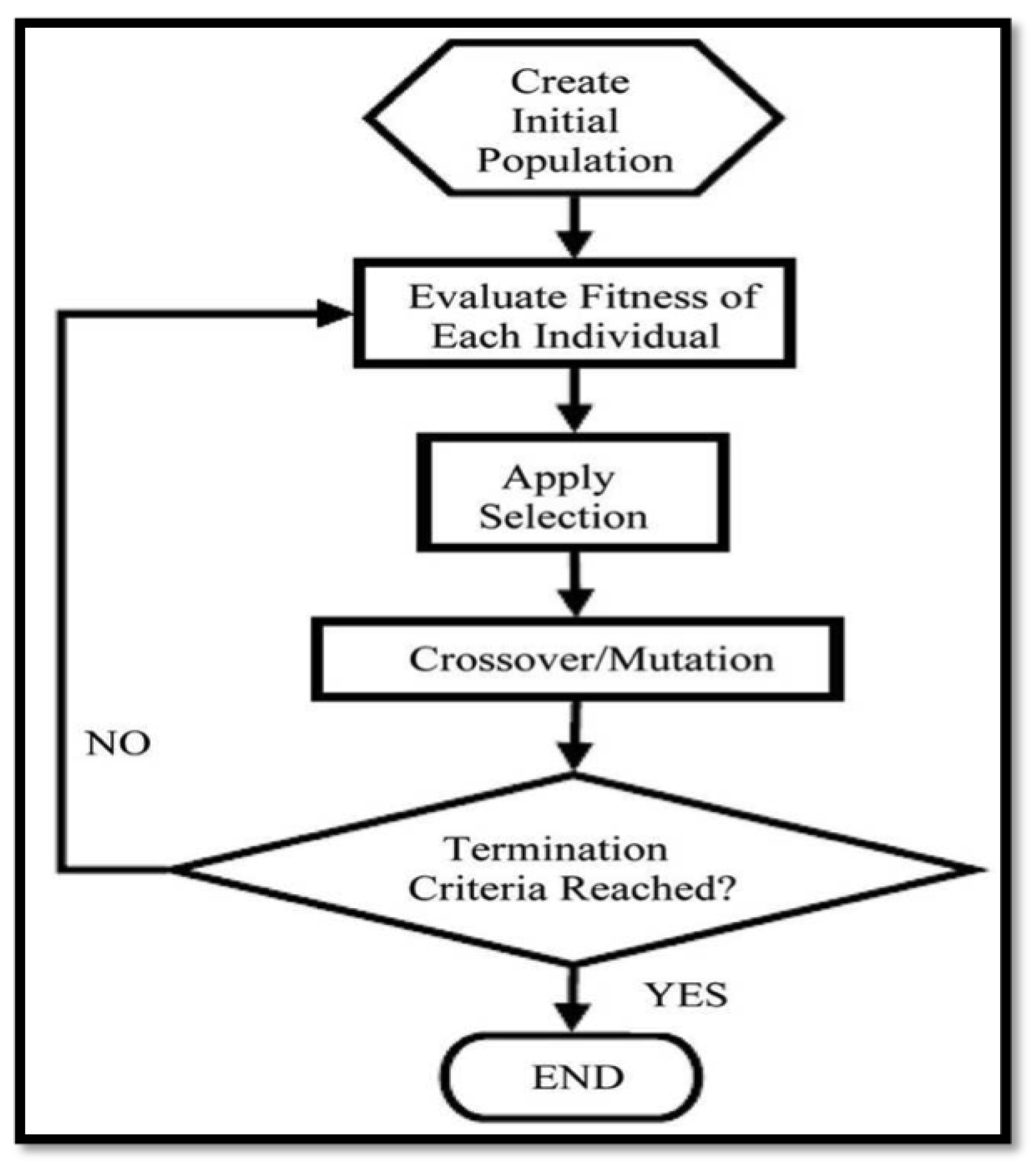
    • Start: Generation of the beginning population of random individuals is the first step of any genetic algorithms. Each generated individual is then represented as a chromosome in a sequence of string with the length L, that aligns with the problem encoding. The step ends with creating a random population in “genotype” [1].
    • Fitness: Next is to compute the fitness value f ( x ) of each individual in the present population. The evaluation process consists of choosing individuals for mating based on their fitness value (parents) and according to the desired values of each. The terms evaluation and fitness are usually used to mean the same thing but it is important to differentiate the evaluating and the fitness valuing as applied in GA. Evaluation function or objective function rates performance based on particular defined aspects. The performance measurement of the fitness function is transformed into a range of reproductive opportunities. [30].
    • New population: Steps 4, 5 and 6 are repeated to create a new population up to completion.
    • Selection (Reproduction): The selection process ascertains the chromosomes that are chosen for mating and reproduction as well as the number of offspring each chosen chromosome produces. The main purpose of the selection process is “the better an individual is; the higher its chance of being a parent” [31]. There exist various traditional selection mechanisms and user-specified-selection mechanisms that are applied in line with the problem in question. [32]. Selection strategies examples consist of:
      (a)
      Tournament Selection: This is arguably the most common selection technique in GA because of its efficiency and ease in implementation [33]. In tournament selection, the selection of individuals is done in a random manner starting with the larger population. Thereafter there is a competition amongst the selected individuals. The competition is used to determine the individual with the highest fitness value to be used in the generation of the new population. The individuals competing are usually set to two also called binary tournament or tournament size. Diversity is ensured in tournament selection as all the individuals have an equal chance to be chosen even though this may reduce the convergence speed. Some of tournament selection advantage includes proper time utilization mostly when the implementation is parallel with low susceptibility to being taken by dominant individuals, and no need for fitness scaling or sorting. [34].
      (b)
      Proportional Roulette Wheel Selection: Also called fitness proportionate. Fitness values are used to choose Parents where the best chromosome stands a higher chance of selection [35,36].
      (c)
      Rank Selection: Parent selection is done using a rank. Here, fitness value is used to rank individuals in the population where the best is ranked (n) and the worst-ranked (1). Every chromosome has a rank depending on its expected value [31].
    • Crossover: The use of the selection process determines the parents used in the crossover to produce a new offspring. Crossover is implemented by selecting a random point on the chromosome where the parents’ parts exchange happens. The crossover then brings up a new offspring based on the exchange point chosen with particular parts of the parents.
      Figure 2a depicts a crossover process [37].
      There are different types of crossover namely: one-point crossover, two-point crossover, and multi-point crossover [39].
      There are some evolving techniques used to accommodate some situations. A brief definition of the two types are as follows:
      (a)
      One-point crossover: One-point crossover works when a crossover point along the chromosome is selected where genes are exchanged between the parents create two offspring (see Figure 2b).
      (b)
      Two-point crossover: Here, two points are selected on the parent chromosomes. There is then the exchange of genes between the two points for the production of two offspring. The crossover operator is used to avoid the exact duplication of the parents from the old population in the new offspring. This ensures that the new population being produced through crossover operation is able to survive in the next generation and also has the desirable parts or qualities of the parents [40].
  • Mutation: Normally, mutation takes place after crossover is done. This operator applies the changes randomly to one or more “genes” to produce anew offspring, so it creates new adaptive solutions good avoid local optima. For example, in binary encoding, one or more randomly chosen bits can be switched from 0 to 1 or from 1 to 0; Figure 2c shows an example.
    Using the crossover operator alone to produce an offspring makes the GA stuck in the local optima, thus, the good parts of the parents survive in each generation, and the local optimal ones are to be found. This problem is called as the local-optima problem. The mutation operator is used to alleviate this problem by proving new offspring different from parents, and this encourages diversity in the population [41].
  • Termination (stopping) criteria: GA at the end must stop to announce the best solution in hand, there are several termination conditions that are used [42], those include:
    1.
    Fixed number of generations reached.
    2.
    The variance of the fitness evolves in the whole population is less than a predefined small quantity (fitness level has been reached [42].
    3.
    No improvement in the best fitness value [21].

2.1. GA Parameters

Determining the interactions that occur among different GA parameters has a direct impact on the quality of the solution, and keeping parameters values “balanced” improves the solution of the GA. There are four basic and important parameters used by GA, those include:
  • Crossover rate (probability): the number of times a crossover occurs for chromosomes in one generation, i.e., the chance that two chromosomes exchange some of their parts), 100 % crossover rate means that all offspring are made by crossover. If it is 0 % , then the complete new generation of individuals is to be exactly copied from the older population, except those resulted from the mutation process. Crossover rate is in the range of [ 0 , 1 ] [43].
  • Mutation rate (probability): this rate determines how many chromosomes should be mutated in one generation; mutation rate is in the range of [ 0 , 1 ] . The purpose of mutation is to prevent the GA from converging to local optima, but if it occurs very often, GA is changed to random search [38,44].
  • Population size: the size of the population indicates the total number of the population’s inhabitants. Selection of population size is a sensitive issue; if the size of the population (search space) is small, this means little search space is available, and therefore it is possible to reach a local optimum. although, if the population size is very large, the area of search is increased and the computational load becomes high [45], therefore, the size of the population must be reasonable.
  • Number of generations: It refers to the number of cycles before the termination. In some cases, hundreds of loops are sufficient, but in other cases we might need more, this depends on the problem type and complexity. Depending on the design of the GA, sometimes this parameter is not used, particularly if the termination of the GA depends on specific criteria.
These GA parameters are determined whether the GA finds an optimal or near-optimal solution, and whether it finds an efficient solution [24]. Any change in the value of these parameters (increasing or decreasing) affects the result of GA negatively or positively [46,47]. Choosing the right parameters is a nontrivial task.

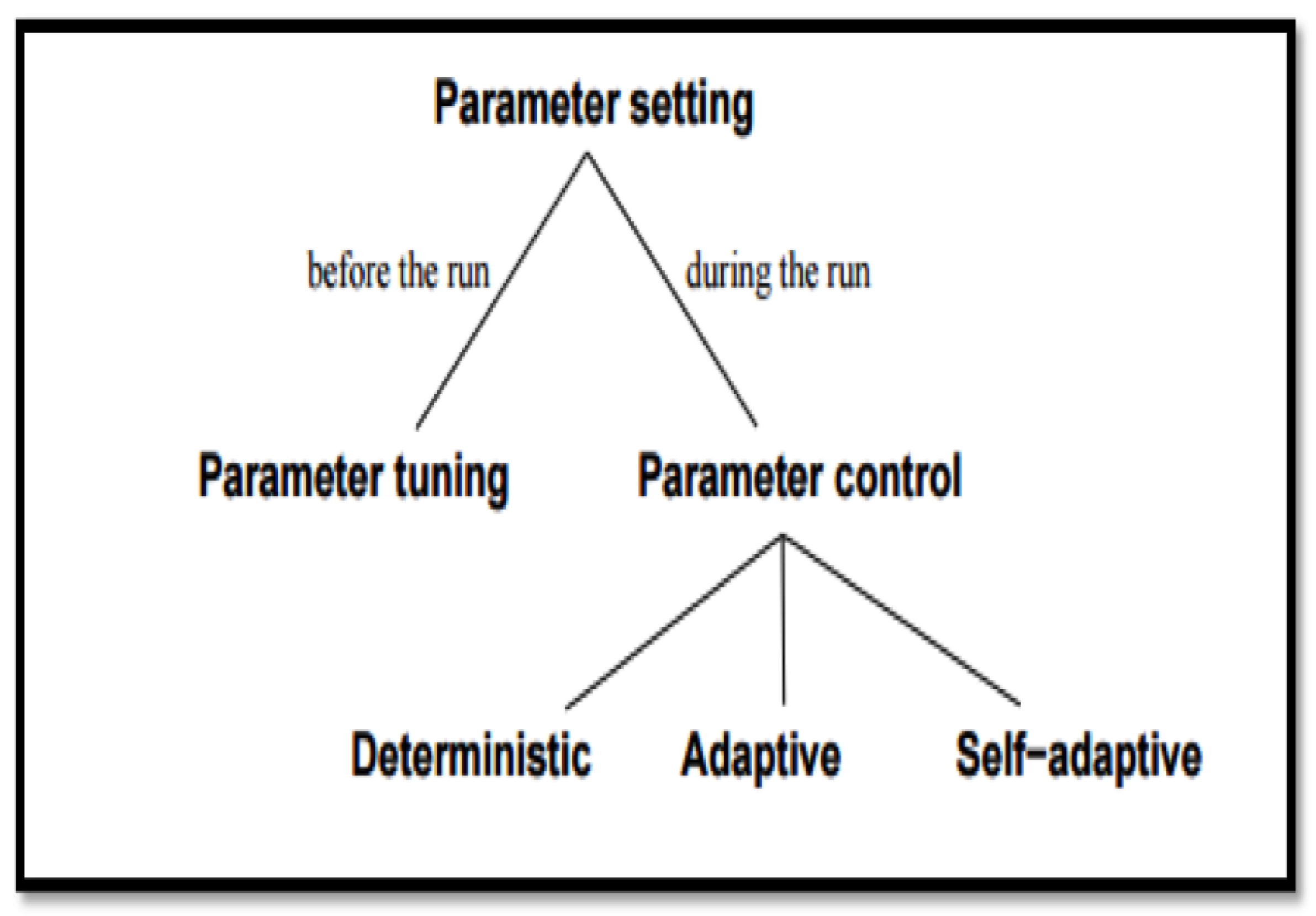
2.2. Crossover and Mutation Ratios

GA involves a process of complex interaction between its parameters, for example: using selection operators alone causes the GA to be stuck in copies of initial population without any new recreation of individuals. However, using selection and crossover operators converges the algorithm to better solutions, but does not guarantee optimality, more likely local optimal (sub-optimal) solutions. Therefore, mutation operator is needed to skip the local search space. Hence, parameters value in GA greatly determines the quality of the final solution [48]. Each operator of GA has a special and different influence. The impact of these factors is influenced by their probabilities, i.e., 100 % probability for crossover gives totally different results from the 50 % . The same applies to mutation probability. Therefore, the GA’s design is limited to a choosing strategy for these parameters [38,48,49]. Keeping a balance between crossover and mutation rates is an issue of controlling parameters in GA. As a matter of fact, controlling values is one of the most important areas of research in GA that has been researched under a main topic known as (parameter setting) [50]. Parameter setting for GA is shown in Figure 3.
There are two main types of setting parameter values, which are classified according to the parameter values behavior during the run: (i) The first one is parameter tuning (common approach), which depends on experimenting the different values for crossover and mutation, and then selecting the ones that give the best results before the final run of the algorithm. This operation is done without any change of the value during the run (fixed value) [50]. (ii) The second type is parameter control, which depends on initial parameter values for crossover and mutation that are changed in somehow in the run process. The techniques for changing the value of a parameter can be categorized to include the following:
  • Deterministic Parameter Control: used when the value of the parameter requires certain modifications using the same outcome rule. The parameter value is tuned to produce the same output without any results from the search process.
  • Adaptive Parameter Control: applied when there is a particular kind of feedback required from the search option that assists in altering the parameter.
  • Self-Adaptive Parameter Control. The GA here is allowed to develop its own parameters. The parameter values to be used are included in the individuals and go through mutation and crossover.
Those types of parameter setting are used by many researchers who attempt to find optimal or near-optimal solutions by using the best rates for crossover and mutation operators. This work fills in this gap, which is finding new strategies for controlling mutation and crossover rates. The proposed methods can be classified as deterministic parameter control.

3. Literature Review for Parameter Selection in GAs

Performance indicators to be used in rating of crossover and mutation are an important aspect in the designing of a GA. The key values of these parameters include; the appropriation of parameters and regulation of parameters. Therefore, over the years, many related works have been proposed to choose the best parameters for GA. In this section, a summary of the most important research conducted in the area is presented. In addition, we review some work related to the traveling salesman problem (TSP), as our proposed methods will be experimented to solve the TSP using GA.

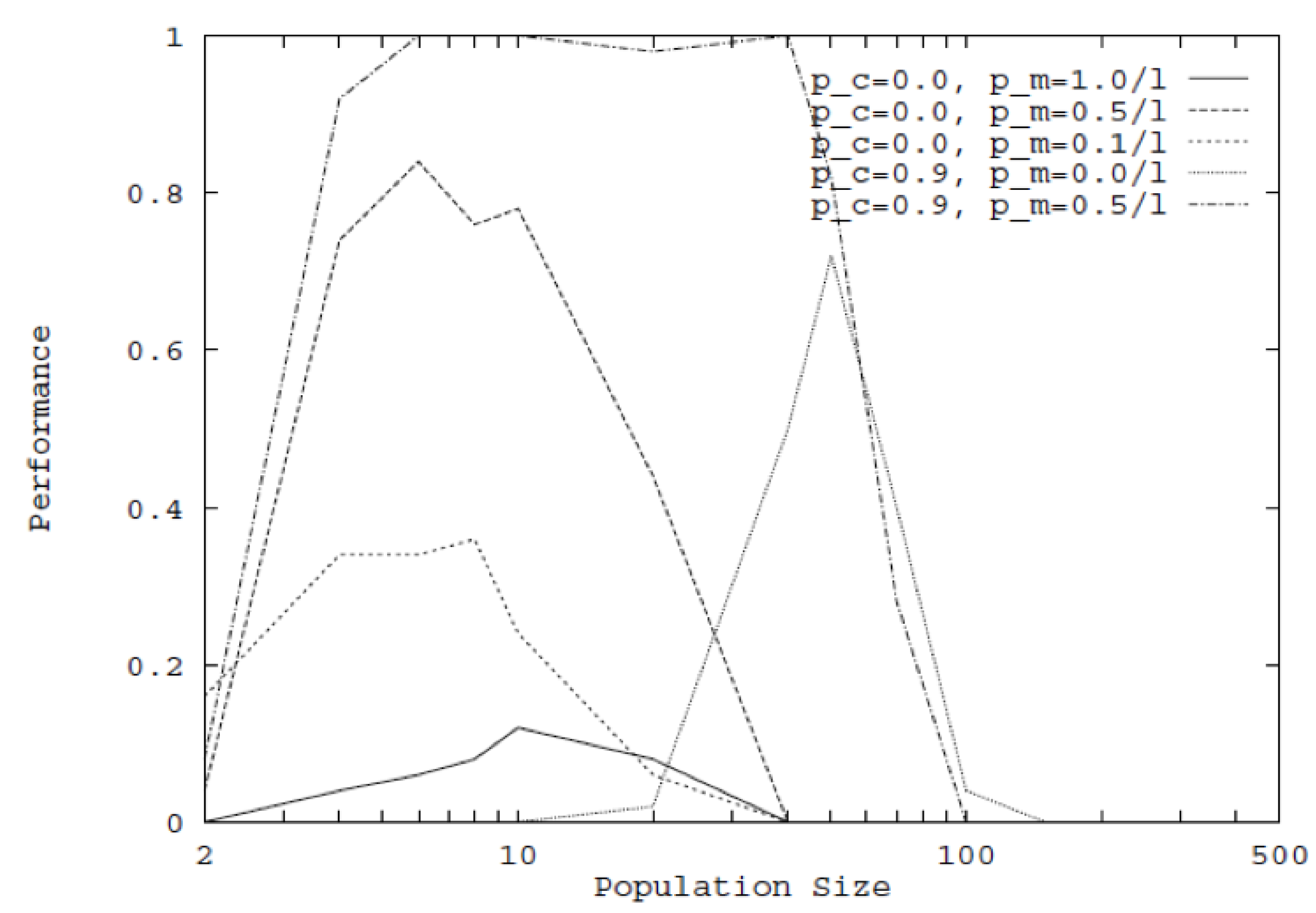
3.1. Crossover and Mutation Rates with Population Size

Since the first mathematically formulated definition of GAs proposed by John Holland in 1975 in his book [1], many studies and pieces of research have been conducted in this field such as [51,52,53].
The crossover and mutation rates was proofed as key elements to success in the search in the GAs [51]. DeJong [54] suggested optimal range values for population size to be in the range of [50–100], mutation parameter rate to be ( 0.001 ), and high mutation rates leads the search to be random, the crossover used was based on one single point crossover to be around the rate of ( 0.6 ). Those parameters have been used in many GA implementations [54].
Grefenstette [32] designed a Meta-GA provided optimal parameters value for the simple GAs, and showed that small population size ranging from (20) to (40) is associated with high crossover rates went in harmony with low mutation rates. In general, his findings revealed that mutation rates above 0.05 were not useful for the optimal performance of (GAs). Accordingly, the researcher suggested another set of parameters with population size value of 30 individuals, a mutation rate of 0.01 and two-point crossover with 0.95 rates [32].
Schlierkamp-Voosen [55] investigated the dynamic behavior of mutation and crossover rates on GA regarding the binary functions. The GA parameter mutation and crossover rates were compared to their optimal solution performance. The mutation rates were most effective in small size populations. While the Crossover rates were depending on the size of the population, and mutation rates were the most robust search in small population size. Nevertheless, the (GA) combined the two operators in such a way that the performance was better than when using a single operator. The (DECEPTION) function showed that increasing the size of the population above to a certain number decreased the quality of the solutions obtained. The analysis of the interaction between mutation and crossover rates showed that the mutation rates normally increased with the size of population. Furthermore, it showed that the mutation rate = 1/n (where n was the size of problem) works efficiently. Using crossover and mutation together, achieved better results than using one of them alone. The crossover appeared to be more efficient than the mutation in larger population size, on the other hand, the mutation was more efficient in small populations [55].
Deb and Agrawal [26] investigated the performance of GA using several experiments that included simple to complex tests for the “onemax” problem. In their work, the researchers compared different (GAs) for several functional evaluations based on calculations and simulation results. The results of the test revealed that for solving simple problems such as “unimodal” or small modality problems, mutation operator played an important role despite crossover rates operator could also solve these problems. However, crossover and mutation rates (when applied alone) had two different effect zones for population size. The first test was conducted using the 0.9 crossover rates, the population size was in the range of (2–500), and a selection operator with (zero) mutation rate. The second test was conducted using the (zero) crossover rate with a population size in the range of (2–500), and with mutation rate of [ 1 , 0.5 , 0.1 ] . The last test combined the two parameters in various values where the mutation rates were [ 1 , 0.5 , 0.1 ] , the two values of crossover rates were [ 0.9 , 0.0 ] . The conclusion of their experiment showed that the selection operators and mutation operators could perform well if accompanied with moderate population size. The selection operators and crossover operators without mutation performed well enough at larger population size than needed for GAs population with selection and mutation operators. In small population size, the researcher concluded that there is a need to use both crossover and mutation parameters as it is shown in Figure 4 [26].
Hong et al. suggested an evolution algorithm called the Dynamic Genetic Algorithm (DGA) to automatically match the crossover and mutation rates according to each individual evaluation results in the new generation. More than one crossover and mutation rates are used simultaneously. The algorithm automatically chose the appropriate crossover and appropriate mutation types. The algorithm is a possible development of GAs performance although the GAs used a one-point crossover process as well a single process of mutation [56].
The population size and its impact on the genetic algorithm were extensively studied. Some researchers seem to agree that small population size could guide the (GA) to poor solutions [57,58,59]. Large population size necessitated that more computation search time was needed in finding an optimal or near optimal solution [59,60]. Rylander and Stanley [61] proposed a new methodology to determine the optimal population size in (GA). They did so by monitoring the difference in the results in each generation in different experiments. The experiments used two types of problems to test, namely the sort problem, and the maximum problem. They used ( 0.1 ) mutation rates, ( 0.5 ) crossover rates and several population sizes (100, 300, 400, 600). The results of the experiments showed the following: First, increasing the population size leads to an increase in the accuracy of the (GA), also the large population size provided a greater chance that the initial state population would contain an individual representing the optimal solution. Second, the large population size resulted in an increase in the number of generations’ convergence [61].
Diaz-Gomez, and Hougen [62] proposed a new approach to find a good initial state population for each small and large populations. The initial population encoded a possible solution to identify the problem. After creating the initial population individuals, each individual was evaluated by fitness value according to the fitness function for the sake of finding a good initial population. The method adopted dealt with small population for the sake of measuring diversity in a small portion of a large size population. They tried as well to generate chromosomes distributed randomly in the fitness landscape by suggesting a new idea using the center of mass, as an alternative method to measure diversity at the population level that depends on the population size, and chromosome length. This approach of analysis and measurement of the diversity of the individuals in the initial random population was important because of the relationship that stood between the initial population and other (GA) parameters and operators [62].
Dong and Wu [63] proposed a dynamic crossover and mutation rates. The crossover rates were calculated dynamically through calculating the Euclidean distance between two chromosomes [64]. They also calculated the Euclidean distance between the greatest and lowest fitness values of the chromosomes in the population. The process of crossover between individuals “long distance individuals” was effective, because of differences that appear among chromosomes, and this would avoid inbreeding and encourage diversity, and thus overcome convergence to local optima [63].
Chiroma et al. [65], conducted a survey of previous approaches and metrics related to the best values of the critical operators that control the quality of solutions. These operators were the mutation rates, crossover rates and the size of the population. They discussed the three operators in terms of decrease or increase in the proportion rates. They also discussed the relationship between mutation rates and crossover rates in the literature search. The small population size indicates insufficient sample sizes, which lead to poor solutions. Large population size indicates high efficiency in the search, and this was better than a small size of population, this also showed slow rate of convergence. The size of the population in this research was in the range of (12–4000). The low crossover rates lead to low rates of exploration. Choosing values between too high and very low crossover rates were to be used for effective implementation of (GA) ranged from ( 0.1 –1). High mutation rates normally led to random search, and the mutation rates were always lower than the crossover rates, in which the mutation rate was in the range of ( 0.001 –1) [65]. The following Table 1 contains GA parameter used to implement GA in previous literature.

3.2. Traveling Salesman Problem (TSP)

TSP is a high-end problem researcher in computer science [90,91,92]. It is simply easy to represent but hard to solve hence categorized under the NP-hard problems [93], which means no solution in polynomial time is discovered so far. A solution to the TSP purposes to obtain the closest path through a number of nodes that have the same start and endpoints in which all nodes are conferred and used once.
Many techniques can be used to solve the TSP, such as [94], (GA) [95,96,97,98], Tabu Search [99], Hill Climbing, Ant Colony [100], Particle Swarm [101], Simulated Annealing [102], Neural Networks [103], Elastic Nets [104], Nearest Neighbor and Minimum Spanning Tree algorithms [105], etc. Potvin [93] and Larrañaga et al. [95] conducted a survey of how to represent the traveling salesman problem (TSP), and also explained the advantages and disadvantages of different mutation and crossover rates and types. Singh and Singh [106] proposed an enhanced crossover operator for solving the traveling salesman problem (TSP).
In his study, Ahmed [107], proposed a method called sequential constructive crossover (SCX) to solve the TSP problem. The basic idea of this method was centered on choosing a point randomly called the crossover point. The method then was employed on sequential constructive crossover before the crossover point by using better edges. The rest of the genes after the crossover site were exchanged between parents to get two children; if there was already a gene, then, it was replaced with an unvisited gene [107].
TSP was considered to be a combination of optimized problems that was simple to describe but hard to solve, and it was categorized as the problems that could not be solved in polynomial time [90] which means it is attached to the NP-hard problems [93]. In 1832 an expert traveling salesman used the term “traveling salesman” in the manual for the traveling salesman that was published in Germany.
We discussed the previous studies that shed light on GA efficiency through developing different parameters of algorithm. Researchers stated that the key to evaluate the process was mainly through showing understanding of the interaction process between the GA parameters namely; crossover rates, mutation rates and population size. These parameters were related to each other in some way that affects the GA efficiency. Many studies agreed that diversity in the initial population with high crossover rates and low mutation rates was the best situation to apply GA. The goal of most of these studies was to bring diversity to the population using crossover and mutation rates to increase the efficiency of the GA.

4. Proposed Dynamic Approach

To improve parametric solutions for a complex system, there are two levels of the problem the system designer and the programmer need to worry about: first level of the problem in which a suitable algorithm is chosen. The second level of the problem, in which various parameters of the chosen algorithm should be chosen carefully to get the highest efficiency. If the chosen algorithm is non-parametric method, there is no need to worry about the second level.
Being a parametric method, GA needs to deal with the second level. When GAs is used in a wide variety of applications and complex systems, the second level task is needed to be applied to control its parameters for the sake of efficiency [32]. As mentioned above, the choice of mutation and crossover rates is well-known to be critical on the behavior and the performance of the (GA).
Many researchers use parameter tuning to set the parameter value in a way that necessitated doing the following: finding the good parameter value before the run (rigid parameters), then running the algorithm using these values. However, other researchers believed that the use of control parameter (Deterministic, adaptive) is more effective to give optimal or near optimal solutions. Some studies recommend using high crossover rates of about 80– 95 % with low mutation rates of about ( 0.1 –1) [38,49].
In another study, the researcher recommends using a high rate of mutation ( 50 % ) with crossover together with small population [26].
Deterministic control parameter modifies the parameter value during the run without any feedback from the search process or user interaction. Accordingly, this type of parameter setting is to be used in an attempt to determine which behavior the parameter should deal with to be effective, and to try to find the optimal or the near optimal solution. Using high crossover rates with low mutation rates alongside large population size refers to the diversity in the large population; however, in the small population size, the mutation rates become lager in order to provide diversity and to increase the search quality [32], bringing diversity to the population using crossover rates and mutation rates to increase the efficiency of the GA.
Next, we propose two deterministic parameter control, followed by discussing two parameter tuning methods to be compared with the proposed methods later.

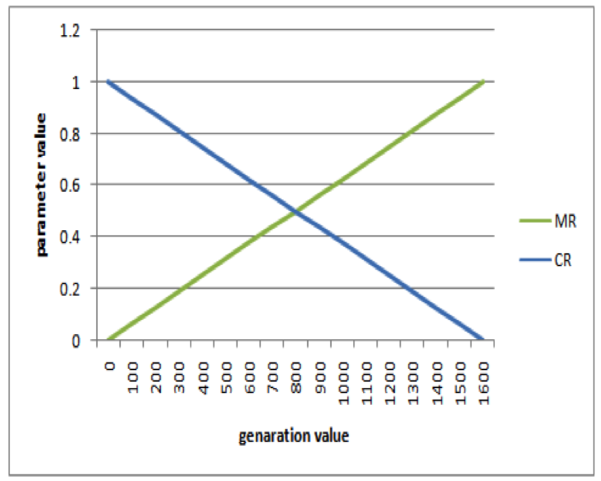
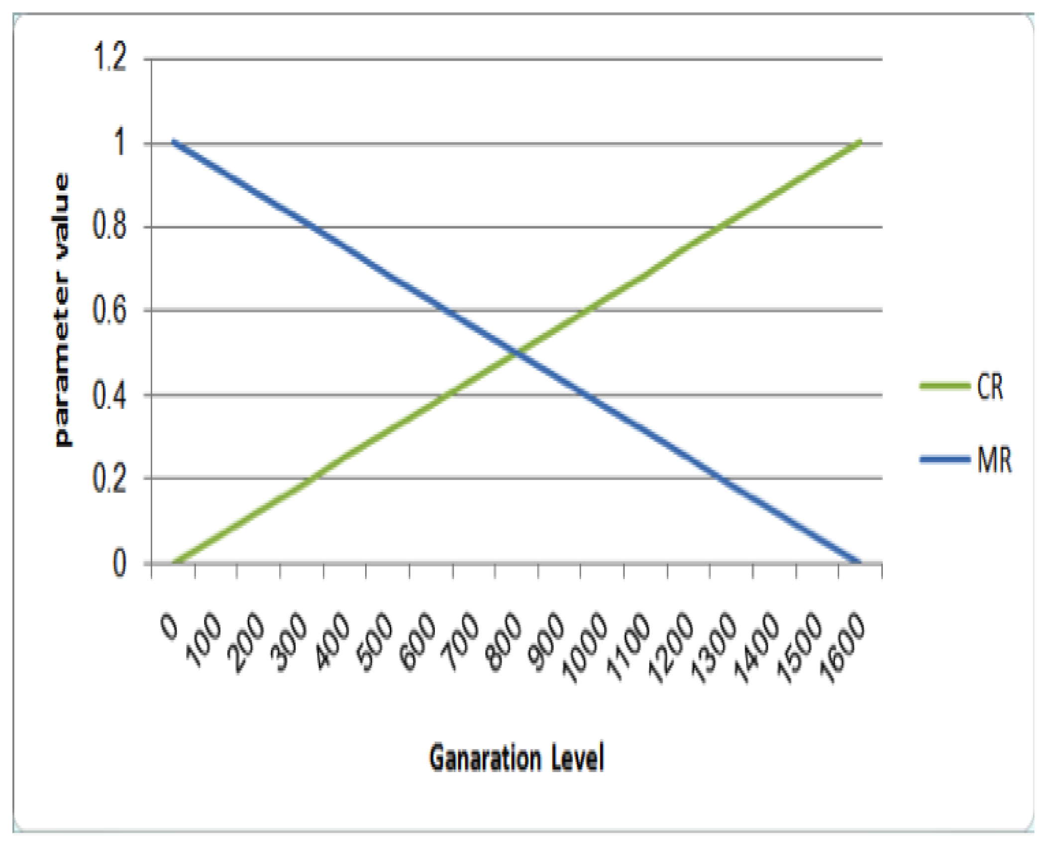
4.1. Dynamic Increasing of Low Mutation/Decreasing of High Crossover (ILM/DHC)

This deterministic method decreases the crossover ratios and increases the mutation ratios (ILM/DHC), where the crossover rate starts to decrease from 100 % to 0 % along the generations, at the same time it increases the mutation rate, which start from 0 % , to be increased linearly to 100 % along the process time.
When the algorithm starts to run Equations (1) and (2) change the mutation rate linearly, step by step according to the total number of generations, and the number of the current generation. To calculate mutation rates in ILM/DHC, the following equation is used:
M R = L G G n where G = [ 1 , 2 , 3 , , G n ] ,
M = M R p o p s i z e ,
where M R is the mutation rate, G n is the total number of generations, L G the number of generation level (the current generation, when the ratio is calculated), M is the number of chromosomes that need to be mutated, “popsize” is population size. At the same time, Equations (3) and (4) change the crossover rate linearly, step by step according to the total number of generations, and the number of the current generation. To calculate crossover rates in (ILM/DHC), the following equation is used:
C R = 1 L G G n ,
C = C R p o p s i z e ,
where C R is the crossover rate, and C is the number of chromosomes that need to be used for the crossover process. This method is used to provide different rates for both crossover and mutation in each generation level. Table 2 and Figure 5 show the rates during the run of GA.
This indicates that the crossover rate is decreased by a specific ratio in each generation level to become to 0 % at the end of the algorithm in last generation. And Mutation rate is increased by a specific ratio in each generation level to reach 100 % at the end of the GA run. As can be seen from Equations (1)–(4) the crossover rate is the complement of the mutation rate at each generation. Figure 5 depicts this relation, and the summation of crossover rate and mutation rate at the same generation level is equal to 100 % . The goal of using dynamic changes in crossover and mutation rates is to bring diversity to the population during the run in a dynamic way.
Example 1.
The value of the mutation and crossover rates are calculated according to the generation level number. If the generation level is 100, the maximum generation = 1600 , and population size is = 100 , then the value of mutation and crossover rates according to Equations (1)–(4) are:
Generation Level = 100 , G n = 1600 , M R = 100 / 1600 = 0.06
M = 0.06 100 = 6 individuals are mutated in generation level 100.
# G e n e r a t i o n = 100 , G n = 1600 , C R = 1 ( 100 / 1600 ) = 0.94
C = 0.94 100 = 94 individuals are used for the crossover process at generation level 100.

4.2. Dynamic Decreasing of High Mutation Rate/Increasing of Low Crossover Rate (DHM/ILC)

This deterministic method is opposite to the ILM/DHC, where the mutation rate is decreased starting from 100 % , and the crossover rate is increased starting from 0 % . By using DHM/ILC when the GA runs Equations (5) and (7) change the rates linearly step by step according to generation number. As can be seen from Table 3 and Figure 6 both of the rates are complement of each other in the same step (generation), where the summation of crossover rate (CR), and mutation rate (MR) in the same generation level is equal to 100 % .
We can calculate the mutation rate in (DHM/ILC) using,
M R = 1 ( l G / G n ) ,
M = M R p o p s i z e ,
and calculate the crossover rate in (DHM/ILC) using,
C R = L G / G n ,
C = C R p o p s i z e .
Example 2.
The values of mutation and crossover rates are calculated according to the generation level number. If the generation level is 500, the maximum generation is = 1600 , and the population size is = 100 , then the value of mutation and crossover rates according to the previous equations are:
L G = 500
G n = 1600
M R = 1 ( 500 / 1600 ) = 0.69
M = 0.69 100 = 69 individuals are to be mutated in generation level 500.
For Crossover rate: L G = 500 , G n = 1600 , C R = ( 500 / 1600 ) = 0.31
C = 0.31 100 = 31 individual are to be used for the crossover process at generation level 500.

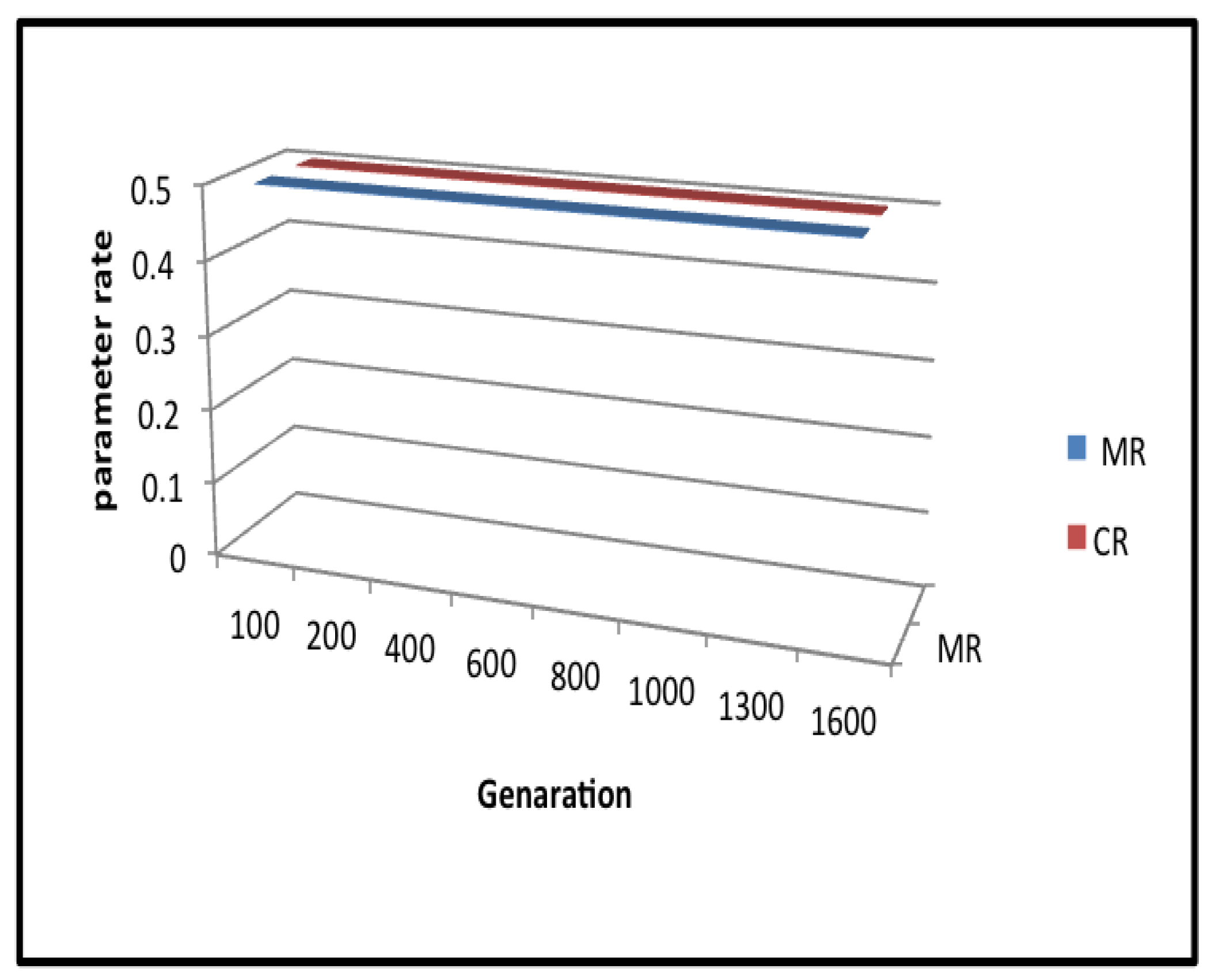
4.3. Fixed 50% for Mutation and Crossover Rates (FFMCR)

Starting from 0 % to 100 % and vice versa makes the average rate (along the run) of mutation and crossover using both DHM/ILC and ILM/DHC is 50 % for each. This motivates us to use a tuning parameter method with the same average rate, thus having the same computation time, and a way to compare the proposed method with a tuning parameter method. These rates were used by some researchers, see for e.g., [88].
The FFMCR uses a fixed ( 50 % ) rate of both mutation and crossover rates. The parameter value in this approach is chosen before the run, and the algorithm continues in running using the same rate. This method shares the same time complexity with the proposed methods. The number of mutated individuals is constant for all generation levels. Also, the number of the crossovers is constant for all generation levels during the run as shown in Table 4 and Figure 7.

4.4. Parameter Tuning Method (0.03 Mutation, 0.9 Crossover) (0.03MR0.9CR)

It is difficult (for the sake of this work) to use all the tuning parameters used in the literature; however, a fixed value for mutation rates is used where MR = 0.03, which is commonly used by some of GAs as explained in the literature review (Section 3), researchers used such rate include and not limited to: [69,72,77]. For the crossover rate we opt for CR = 0.9, because most of the GAs found in the literature used high rate for crossover, were most of the used CR in the range of 0.5 to 0.9 . Researchers who used such rate include and not limited to: [69,83,84,86,87]. The number of mutated individuals is constant for all generation levels, also the number of individuals participated in crossover is constant for all generation levels during the run. We used the 0.03MR0.9CR as base for comparing our proposed work.
We proposed and discussed two new deterministic approaches for choosing mutation and crossover rates dynamically, namely DHM/ILC and ILM/DHC, in addition, two “parameter tuning” approaches to the same problem is presented, namely FFMCR and 0.03MR0.9CR, these were discussed to be compared with the proposed method in terms of solution goodness, and computational time consumed. Next, we provide detailed experimental results and discussion of our proposed dynamic approaches for the parameter selection in GAs.

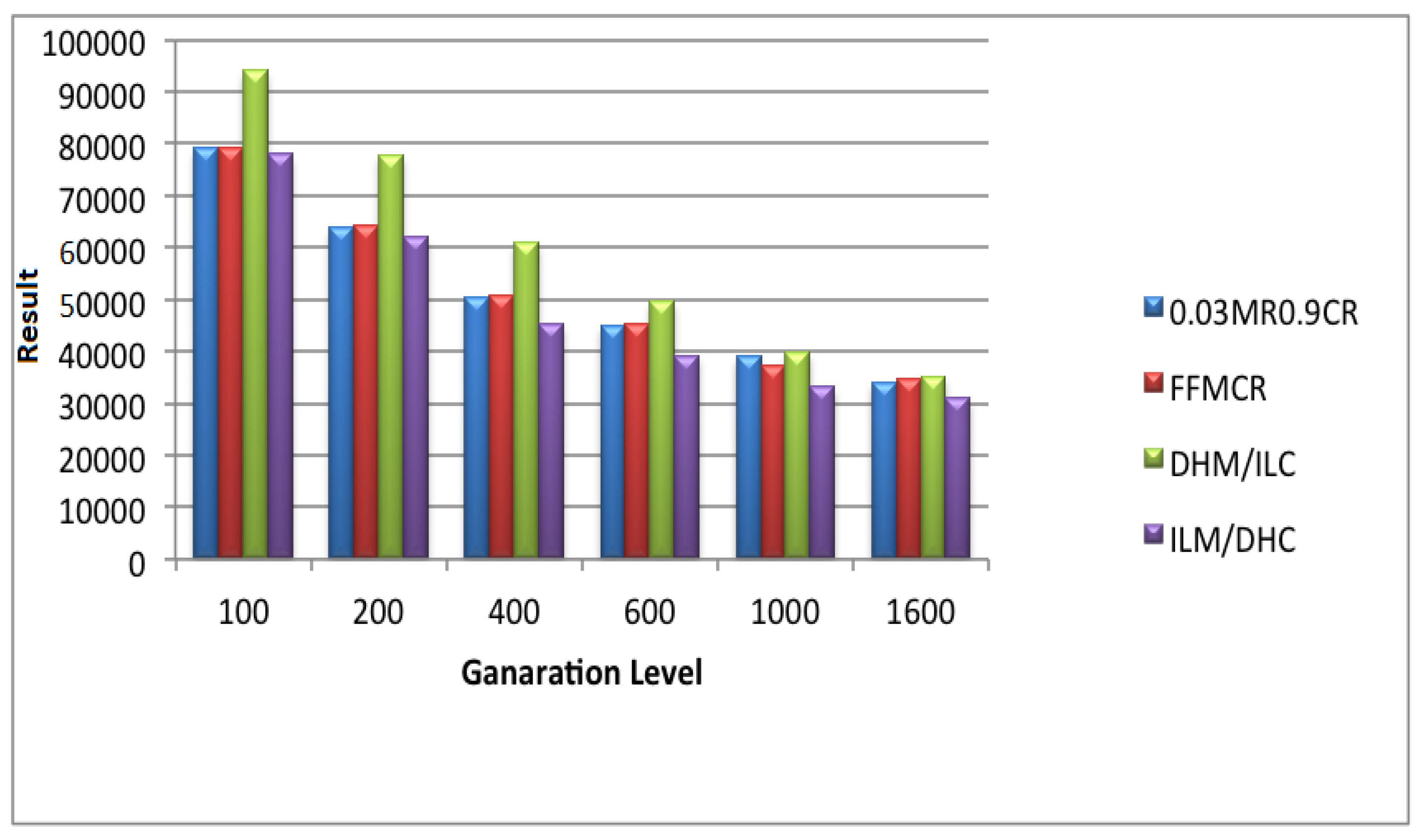
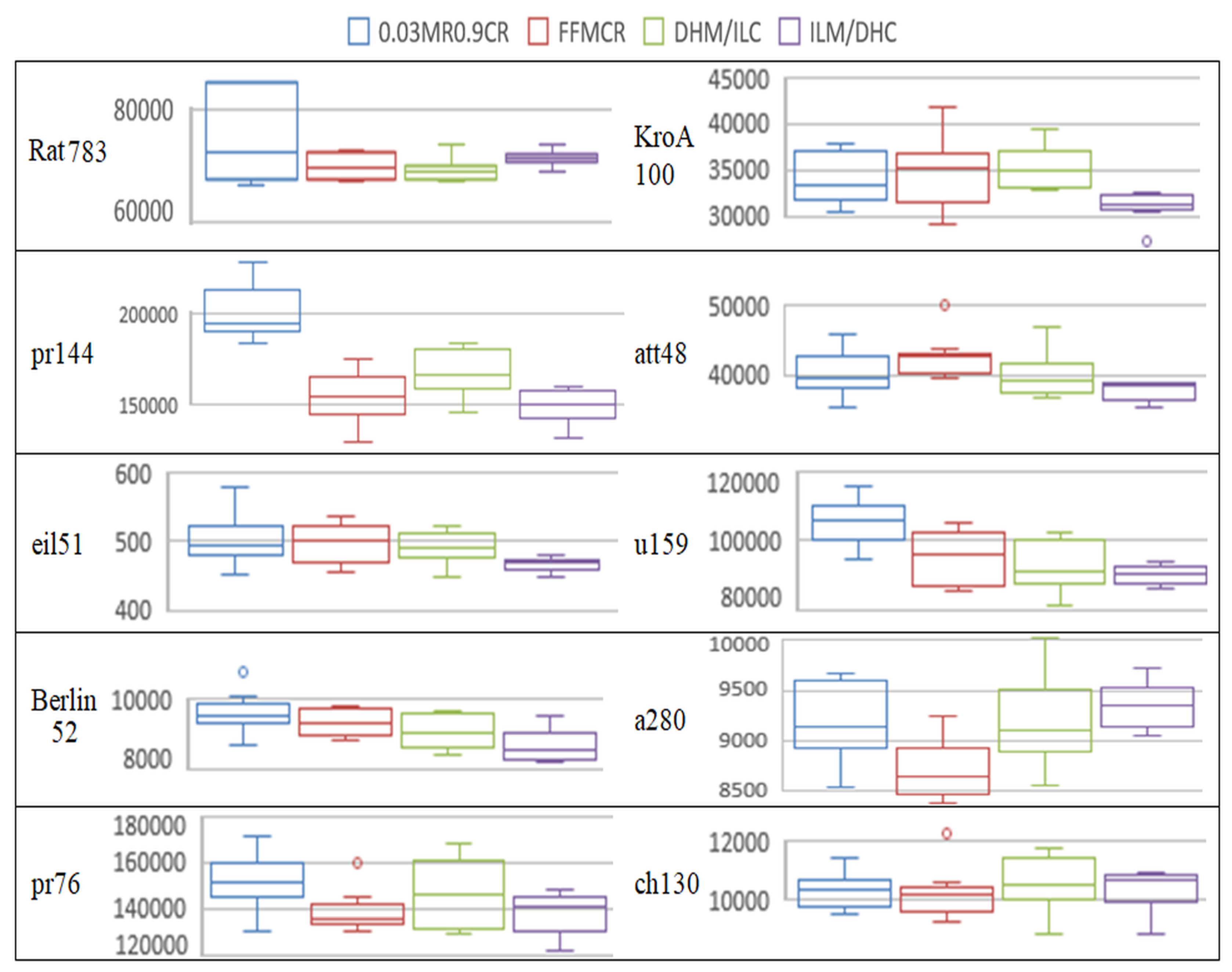
5. Experimental Results and Discussion

Six sets of experiments were conducted to evaluate the proposed methods based on on the population size on different TSP problems; each set of experiments used four types of parameter settings, the proposed deterministic approaches; which are DHM/ILC and ILM/DHC. In addition, two parameter tuning approaches; namely FFMCR and 0.03MR 0.9CR. Different sizes of the population used to investigate the effect of the population size on the results using different parameter setting approaches. Population sizes used:
(1)
Small population size (25 and 50); sets 1 and 2.
(2)
Moderate population size (100 and 200); sets 3 and 4.
(3)
Large population size (300 and 400); sets 5 and 6.
According to all the experiments, GA applied the reinsertion technique that is essentially sampling [63], where desirable qualities from both the new and the old generation individuals are chosen to be the population for the next generation. That is there is competition between the old and the new individuals.
The initial population seeding in all algorithms is random, and the selection strategy is a roulette wheel. The fitness function used by GA is a problem dependent; here we used the total distance of the TSP route, i.e., the summation of the distances between the sequence instances along the chromosome, the “best” solution is characterized by the minimum total distance, since the TSP is a minimization problem. The mutation operator used for all experiment sets is the exchange mutation [108]: which selects two genes randomly and switch between their positions. The crossover operator used is the Modified Crossover [109]. This crossover operator is an extension of the one-point crossover, which chooses the cut point at random from the first parent; then, the first child is created by appending genes (before cutting point) in the second parent to the first part. Finally, it repairs the rest of the gene to prevent duplicates. The termination criteria are based on a fixed number of generations reached, for all our experiments, the maximum number of generations was set to 1600. We used Path representation for encoding the TSP, where there is a natural representation for the tour [110], for example: a tour of city1 -> city3 -> city4 -> city2 -> city1 is represented in an integer array containing the cities’ indexes: (1, 3, 4, 2).
The data set used for all sets of experiments includes 10 real TSP data; namely a280, u159, ch130, kroA100, pr76, berlin52, att48, eil51, pr144 and rat783, which were taken from the TSPLIB [111]. The number at the end of the name of each TSP indicates the number of instances (cities), each city is identified by its (x, y) location and a sequence number as shown in Figure 8. The chromosome, in this case, has random sequential numbers meaning that the chromosome length depends on the problem size n that is the size of each TSP problem. The result of the GA is the best solution that can be obtained, which is (in our case) the minimum total tour length, the word “result” and the “minimum total tour length” will be used interchangeably in this paper.

5.1. Set 1 of Experiments (Population Size = 25)

The aim of this experiment is to measure the performance of the proposed methods (DHM/ILC and ILM/DHC), compared to the tuning parameter approaches (0.03MR0.90CR and FFMCR) under a constant population size of 25 solutions (chromosome) for all the runs.
The GA is applied ten times, and the average of its “best” converged solution at each generation is recorded, starting from generation 100 up to generation 1600. Convergence to an optimal solution is beyond the purpose of this paper; however, we mean by convergence that the algorithm is providing better solutions while the generation number is increased.
Results from the first set of experiment showed that the best performance was recorded by the dynamic (ILM/DHC) rule, the “best performance” means here the ability to find the best solution on average, and the best solution is the minimum feasible rout for each TSP data. In most cases the performance of the dynamic (ILM/DHC) rule was better than the performance of the other methods, as is shown in Figure 9 and Figure 10. The results of GA using different parameter setting methods on different TSP data are shown in Table 5 and Figure 11.
As can be seen from Table 5 and Figure 11, the results indicate the efficiency of the Dynamic ILM/DHC over the other methods, where the Dynamic ILM/DHC performed the best in seven problems: pr76, berlin52, kroA100, att48, eil51, u159 and pr144, followed by the FFMCR, which performed the best in two problems: a280 and ch130. In this experiment, the population size is small (25), i.e., the diversity is not maintained we think that the Dynamic ILM/DHC provides diversity in small population, because starting the GA with a large crossover rate and small mutation rate with such a small population size, create similar offspring; however, while generation level goes up, the mutation rate become larger, and bring up different offspring, allowing the GA to skip local optima. this claim is also supported by the results from Figure 9 and Figure 10, where the ILM/DHC started to take the lead significantly after generation 600 (Figure 9 and Figure 10) that is acceptable, as a higher mutation rate is used, since in a small population higher mutation rate is needed to provide more diversity, to the small population, which had limited search space with just 25 individuals. The mutation started to be higher and more effective in generation (1000) to end the GA wining all the other methods.

5.2. Set 2 of Experiments (Population Size = 50)

The results from the second set of experiments showed that the best performance was also recorded by the Dynamic ILM/DHC rule, as we are still talking small population In most cases, the performance of the dynamic (ILM/DHC) rule was better than of the performance of the other method as is shown in Figure 12 and Figure 13. The results of GA using different parameter setting methods on different TSP data with population size = 50 individuals are shown in Table 6.
As can be seen from Table 6, the results indicate the efficiency of the Dynamic ILM/DHC over the other methods where the Dynamic ILM/DHC provided the best solutions to: pr76, berlin52, kroA100, att48, eil51, u159, a280 and ch130 followed by FFMCR that performed the best on: rat783, pr144.
In this set of experiments, the population size is still small (50). Therefore, we stick with the aforementioned explanation of the efficiency of the proposed ILM/DHC when it is applied on small populations. Results from Figure 12 and Figure 13 also supports the same explanation, as ILM/DHC approach started to take the lead after (1000) generations, i.e., a higher mutation ratio to support diversity.

5.3. Set 3 of Experiments (Population Size = 100)

The results from the third set of experiments show that the best performance result was recorded by the dynamic (ILM/DHC) approach. In most cases, the performance of the dynamic (ILM/DHC) rule was better than of the performance of the other method as is shown in Figure 14 and Figure 15. The results of GA using different parameter setting methods on different TSP data with population size = 100 individuals are shown in Table 7.
As can be seen from Table 7, the results still indicate the efficiency of the Dynamic ILM/DHC over the other methods where the Dynamic ILM/DHC provided the best solutions to: pr76, kroA100, att48, sh130, and pr144, followed by FFMCR berlin52, u159 and a280, followed by DHM/ILC, which started to perform better compared to smaller populations In this experiment, the population size is moderate (100), and therefore, the ILM/DHC did not perform better than it used to do in smaller populations, in addition, the difference in the quality of the provided solutions from the other methods is not significant (see Figure 14 and Figure 15), and only won 5 TSPs, this means that the ILM/DHC started to lose some of its reputation as we increase the size of the population, since diversity is partially maintained in moderate population sizes. According to the results of the previous three sets of experiments, the Dynamic ILM/DHC recorded the best results in small sized populations (25, 50), nevertheless it start to become weaker in moderate sized populations (100). This triggers the following question: What if the population size got larger?
The answer of this question we need further sets experiments using larger population sizes.

5.4. Set 4 of Experiments (Population Size = 200)

The results of the fourth set of experiments show that the best performance was recorded by the Dynamic DHM/ILC approach. In most cases, the Dynamic DHM/ILC outperformed the other approaches as shown in Figure 16 and Figure 17. The results of GA using different parameter setting methods on different TSP data with population size = 200 individuals are shown in Table 8.
As can be seen from Table 8, the results indicate the efficiency of the Dynamic DHM/ILC over the other methods where the Dynamic DHM/ILC performed the best solution to the problems: pr144, pr76, eil5, berlin52, att48, followed by the FFMCR and the ILM/DHC that performed the best in two problems in addition. A population with 200 individuals is a large population. In addition, therefore the diversity is almost maintained, and GA does not need high mutation rate to increase diversity, on the contrary it needs more crossovers to generate better offspring from the diverse large sized population, particularly, when the GA process goes to higher level of generations. This result is expected, since we noticed the degradation in the performance of the ILM/DHC as the population size goes larger, knowing that the ILM/DHC approach is opposite to the DHM/ILC approach.

5.5. Set 5 of Experiments (Population Size = 300)

The results from this set of experiments show that the best performance is also recorded by the Dynamic DHM/ILC approach. In most cases the performance of the Dynamic DHM/ILC was better than of that of the other approaches, this is shown in Figure 18 and Figure 19. The results of GA using different parameter setting methods on different TSP data with population size = 300 individuals are shown in Table 9.
As can be seen from Table 9, the results indicate the efficiency of the Dynamic DHM/ILC over the other approaches where the Dynamic DHM/ILC performed the best solutions for the problems: rat783, pr76, eil51, berlin52, KroA100, ch130, u159, a280 and pr144 followed by the Dynamic ILM/DHC in problem: att48. This show the domination of the DHM/ILC in larger populations and support the previous set of experiments, giving more stable results as increasing the size of the population, the aforementioned explanation still applies for the same mentioned reasons.

5.6. Set 6 of Experiments (Population Size = 400)

The Results from this experiment shown that the best performance is still recorded by the Dynamic DHM/ILC approach. In all the tested cases, the performance of the Dynamic DHM/ILC was better than those of other approaches, the performance of all approaches is shown in Figure 20 and Figure 21. results are averaged over 10 runs. The results of GA using different parameter setting methods on different TSP data with population size = 300 individuals are shown in Table 10.
As can be seen from Table 10 and Figure 22, the results indicate the superiority of the Dynamic DHM/ILC over all the other approaches, where the Dynamic DHM/ILC provided the best solution for all problems used in the experiments. Moreover, the provided solutions are significant compared to the other approaches, i.e., the difference between the best solutions (provided by the DHM/ILC) and the other solutions (provided by other approaches) is high and significant. Same explanation provided in the previous sets of experiments applies here, the only difference is that the population size has become larger (400), and therefore the diversity is guaranteed, so the need for more crossovers at the end of the GA is vital, and much important that the number of mutations, which yields diverse but weak solutions, while the crossover yields stronger solutions as larger parts of the “good” chromosomes are exchanged to provide even better individuals. Another thing that worth mentioning is the result of the most common approach for GA parameter setting, which is the 0.03MR0.9CR, this approach was used extensively by researchers who used GA for solving optimization problems, we found with this number of experiment that this approach never won any problem except one problem (rat783) in experiment set 4 with population size 200.
More results from the six sets of experiments can be seen at Appendix A.

5.7. Time Complexity

Time complexity of the proposed work in comparison with other methods. The time complexity of the (GAs) depended mainly on the representation of the chromosomes (the size of the chromosome, which varied depending on the problem), the genetic parameters (number of generations, population size, mutation probability and crossover probability), and the selection time [30]. Consequently, the time complexity of the (GA) is calculated as follows: Suppose that the size of population is (P), the number of generations is (G), the probability of crossover and mutation were (PC and PM) respectively, and the chromosome size is (n), which is the variable number of instances (TSP cities in our case), normally,
n > > a c o n s t a n t .
The Quick Sorting algorithm is used to sort out the population and to take the best solutions. The number of operations needed for the selection process was:
( P × log ( P ) )
The number of the mutated chromosomes was equal to
( P M × P ) .
Since we need to go along each chromosome; the number of operations needed for the mutation process is:
( P M × P × n )
The number of crossovers is equal to
( P C × P )
However, Crossover operator is a binary variation operation, i.e., it works on 2 chromosomes, and yield two chromosomes (offspring), while the mutation operator is a unary variation operator, works on one chromosome and yield only one chromosome, therefore The number of crossovers is equal to
( 2 × P C × P ) .
Since we need to go along each chromosome; the number of operations needed for the crossover process is:
( 2 × P C × P × n ) .
All the previous operations were repeated (G) times. Therefore, the time complexity of the overall (GA) is:
T = G ( ( P × log ( P ) ) + ( P M × P × n ) + ( 2 × P C × P × n ) )
Since, G and P were constant (ks) regardless of what the problem was, assuming that k 1 = G , k 2 = P , k 3 = P M × P , k 4 = P C × P then theoretically: k = k1 = k2 = k3 = k4, and therefore (GA)TC became:
T = k ( ( k × log ( k ) ) + ( k × n ) + ( k × n ) )
= k 2 log ( k ) + 2 n k 2
Since k was a constant, then k 2 and log ( k ) were also constants, which makes the Equation (10) as the following:
T = k + ( k n )
Therefore, the time complexity of the traditional (GAs) is linear (of order (n)), i.e., T depended mainly on the problem size (chromosome size) as it is the only variable in the process:
T = O ( n )
However, in practice, we feel that some approaches are slower than others, so we need to analyze the time complexity of the four approaches depending on Equation (9). Assume that time complexity for DHM/ILC is T1, and time complexity for ILM/DHC is T 2 . The average of crossover rates used by DHM/ILC is
A V = ( 0 % + 1 % + 2 % + + 100 % ) / 100
= ( 100 ( 100 + 1 ) / 2 100 ) / 100
According to the Gaussian closed form
A V = ( 100 ( 100 + 1 ) / ( 2 100 ) / 100 = 50 %
And the average of the mutation rate is the same; hence they are complements of each other, and
T 1 = T 2
Because they have the same ratios but opposite to each other Recalling Equation (9) we get,
T 1 = T 2 = G ( ( P × log ( P ) ) + ( 50 % × P × n ) + ( 2 × 50 % × P × n ) ) = G × ( ( P log ( P ) ) + ( 1.5 P × n ) )
Assuming that T3 represents time consumed by FFMCR, since it uses 50
T 3 = T 1
Assuming that T4 represents the time consumed by 0.03MR0.9CR, recalling Equation (9) we get,
T 4 = G ( ( P × log ( P ) ) + ( 3 % × P × n ) + ( 2 × 90 % × P × n ) ) = G × ( ( P log ( P ) ) + ( 1.74 P × n ) )
As can be seen from Equations (14) and (15), the number of operations needed by the proposed method is less than those of the 0.03MR0.9CR, and therefore the proposed approaches for choosing the mutation and crossover ratios is faster than the most common predefined rates (0.03MR0.9CR).

6. Conclusions

We reviewed GA representations and parameter selection in GAs along with new deterministic approaches were proposed to change the crossover and mutation rates parameters dynamically. Without any feedback or user interaction, the change in parameters value linearly based on mathematical equations, namely ILM/DHC and DHM/ILC. Based on several sets of experiments on real data from the TSPLIB, the Dynamic ILM/DHC was the best to operate with small population size, attaining the best solutions if compared with FFMCR, 0.03MR0.9 CR and DHM/ILC in small population (25, 50, 100). The success of this algorithm in small sized population is due to lack of diversity of such small search space, and therefore, by the increasing level of generation, and the extensive use of crossover operations the final solutions become almost similar, and in need for a large number of mutations, which is provided to the GA just on time, preventing the algorithm from stuck at a local optima, and therefore increases the performance of the GA with small sized population. The results also showed that the Dynamic DHM/ILC performed very well with large population sizes (200, 300, 400) if compared with other methods. this is due to the need for more crossovers at the end of the algorithm at higher levels of generation, as the large sized populations are diverse by nature, and therefore do not need many mutations to get the algorithm from a local optima, on the contrary it needs more stronger solutions that depends on exchanging larger parts from good parents to provide better offspring, and this enhance the final solution of the GA with large populations.
We note also that the 0.03MR0.9CR approach (which is one of the most used predefined parameter setting) did not perform the best in any set of experiments, nor with any population, so we think that using such predefined rates for both crossover and mutation is not a good practice, in terms of quality of solutions and time complexity. In the future, we intend to extend the proposed approaches to be used for GA parameter setting for other optimization problems, such as the maxone, the knapsack problem, scheduling problems, etc.
The experimental results show averages across 10 runs, and we draw conclusions from small differences in these averages. If the scatter is too strong, these conclusions might not be well-founded, therefore, we plan to increase the number of runs to be at least 30 runs for each experiment in the future. Moreover, the linearity of the approaches needs to be further investigated, and compared with other adaptive and self-adaptive approaches, in addition to use indexing techniques such as [112,113,114,115].

Author Contributions

Conceptualization, A.H. (Ahmad Hassanat) and E.A. (Esra’a Alkafaween); methodology, A.H. (Ahmad Hassanat) and K.A. (Khalid Almohammadi); software, A.H. (Ahmad Hassanat); validation, E.A. (Eman Abunawas), E.A. ( Esra’a Alkafaween) and K.A. (Khalid Almohammadi); formal analysis, A.H. (Awni Hammouri) and V.B.S.P.; investigation, E.A. (Eman Abunawas); resources, E.A. (Eman Abunawas); data curation, E.A. ( Esra’a Alkafaween); writing—original draft preparation, A.H. (Ahmad Hassanat) and V.B.S.P.; writing—review and editing, K.A., A.H. (Ahmad Hassanat) and V.B.S.P.; visualization, E.A. (Eman Abunawas); supervision, A.H. (Ahmad Hassanat); project administration, A.H. (Ahmad Hassanat).

Funding

This research received no external funding.

Conflicts of Interest

The authors declare no conflict of interest.

Appendix A. Results from the 6 Sets of Experiments Conducted for this Study

More results from the 6 sets of experiments conducted for this study are given below in Table A1, Table A2, Table A3, Table A4, Table A5,Table A6, Table A7, Table A8, Table A9 and Table A10.
Table A1. The solution average in TSP (berlin52) problem, four ratios with several population sizes.
Pop SizeGenerationDynamic DHM/ILCDynamic ILM/DHC0.03MR0.9CRFFMCR
40016008619.791669250.79167.6
30016008790.792079642.69136.7
20016009052.39526.99697.69397.8
10016008782.58820.19200.38667.2
5016009166.39024.594649155
2516009068.28637.49606.19314.8
Table A2. The solution average in TSP (pr76) problem, four ratios with several population sizes.
Pop SizeGenerationDynamic DHM/ILCDynamic ILM/DHC0.03MR0.9CRFFMCR
4001600135,876.6141,485.1152,704.2142,986.3
3001600133,732.8140,053.7159,528.7146,208.2
2001600139,640.5142,065.1151,172.8149,717.8
1001600149,661.5139,733.7148,600.5146,552.8
501600139,644.6135,316.6155,182.4140,766.9
251600146,682.1138,070.6151,834.4138,614.6
Table A3. The solution average in TSP (KroA100) problem, four ratios with several population sizes.
Pop SizeGenerationDynamic DHM/ILCDynamic ILM/DHC0.03MR0.9CRFFMCR
400160030,804.132,291.936,751.334,094.3
300160031,003.131,39535,14332,257.4
200160032,754.532,435.634,587.635,331.6
100160032,549.231,598.734,19132,176.1
50160032,058.631,630.639,674.832,730.7
25160035,236.831,084.934,126.134,881.2
Table A4. The solution average in TSP (u159) problem, four ratios with several population sizes.
Pop SizeGenerationDynamic DHM/ILCDynamic ILM/DHC0.03MR0.9CRFFMCR
400160087,507.696,255.1101,313.294,858.3
300160091,893.996,699.195,409.894,542.2
200160091,861.192,766.494,578.191,125.4
100160095,826.598,65998,011.690,671.5
50160095,642.693,439.5101,332.393,621.9
25160092,659.690,066.3105,187.994,397.3
Table A5. The solution average in TSP (ch130) problem, four ratios with several population sizes.
Pop SizeGenerationDynamic DHM/ILCDynamic ILM/DHC0.03MR0.9CRFFMCR
40016009854.910,62211,526.710,247.1
3001600991210,68713,084.610,364.4
200160010,687.210,213.410,442.910,238.1
100160010,253.310,192.411,48010,609.8
50160010,383.210,178.511,455.410,231.1
25160010,60510,366.310,315.110,235.4
Table A6. The solution average in TSP (a280) problem, four ratios with several population sizes.
Pop SizeGenerationDynamic DHM/ILCDynamic ILM/DHC0.03MR0.9CRFFMCR
40016008698.49862.19287.79177.3
30016008645.69352.69017.89031.9
20016009175.89425.49504.48912.6
10016009134.19457.78957.18897
5016009295.99067.39304.79264.5
2516009176.59364.19180.78703.6
Table A7. The solution average in TSP (att48) problem, four ratios with several population sizes.
Pop SizeGenerationDynamic DHM/ILCDynamic ILM/DHC0.03MR0.9CRFFMCR
400160036,854.539,310.443,077.141,121.3
300160038,628.138,613.440,653.140,671.7
200160036,502.138,514.740,504.640,272
100160037,355.836,929.541,811.139,459.3
50160038,448.137,244.239,872.240,686.3
25160039,909.637,507.340,044.242,510.5
Table A8. The solution average in TSP (eil51) problem, four ratios with several population sizes.
Pop SizeGenerationDynamic DHM/ILCDynamic ILM/DHC0.03MR0.9CRFFMCR
4001600476.6485.4519.6498.7
3001600475.1494.2521.9496.3
2001600468.5481.6501.5490.7
1001600479483.1496.8481.1
501600486472.5511.1488.4
251600491.7465.4501496.8
Table A9. The solution average in TSP (pr144) problem, four ratios with several population sizes.
Pop SizeGenerationDynamic DHM/ILCDynamic ILM/DHC0.03MR0.9CRFFMCR
4001600146,385.7158,169.1174,357.6149,038.5
3001600148,610.7157,487.6178,213.8149,154.5
2001600155,994.3165,080.7169,101.1177,072.5
1001600156,527.1153,154.0172,820.9158,910.4
501600157,446.3151,455.1175,095.8151,072.1
251600167,311.4146,634.9200,770.7154,258.6
Table A10. The solution average in TSP (rat783) problem, four ratios with several population sizes.
Pop SizeGenerationDynamic DHM/ILCDynamic ILM/DHC0.03MR0.9CRFFMCR
400160067,424.373,022.871,517.669,253.6
300160068,091.972,438.569,554.870,979.8
200160067,399.371,571.370,486.371,100.3
100160067,795.771,098.270,183.668,322.4
50160068,424.371,127.776,42867,791.5
25160069,123.671,432.379,75269,843.1

References

  1. Holland, J.H. Adaptation in Natural and Artificial Systems: An Introductory Analysis with Applications to Biology, Control, and Artificial Intelligence; MIT Press: Cambridge, MA, USA, 1975. [Google Scholar]
  2. Man, K.F.; Tang, K.S.; Kwong, S. Genetic algorithms: Concepts and applications. IEEE Trans. Ind. Electron. 1996, 43, 519–534. [Google Scholar] [CrossRef]
  3. Golberg, D.E. Genetic Algorithms in Search, Optimization, and Machine Learning; Addison-Wesley: Boston, MA, USA, 1989. [Google Scholar]
  4. Whitley, D. A genetic algorithm tutorial. Stat. Comput. 1994, 4, 65–85. [Google Scholar] [CrossRef]
  5. Tsang, P.W.M.; Au, A.T.S. A genetic algorithm for projective invariant object recognition. IEEE TENCON Digit. Signal Process. Appl. 1996, 1, 58–63. [Google Scholar]
  6. Mohammed, A.A.; Nagib, G. Optimal routing in ad-hoc network using genetic algorithm. Int. J. Adv. Netw. Appl. 2012, 03, 1323–1328. [Google Scholar]
  7. Srivastava, P.R.; Kim, T.H. Application of genetic algorithm in software testing. Int. J. Softw. Eng. Its Appl. 2009, 3, 87–96. [Google Scholar]
  8. Paulinas, M.; Ušinskas, A. A survey of genetic algorithms applications for image enhancement and segmentation. Inf. Technol. Control 2015, 36, 278–284. [Google Scholar]
  9. Hassanat, A.B.; Prasath, V.S.; Mseidein, K.I.; Al-Awadi, M.; Hammouri, A.M. A HybridWavelet-Shearlet Approach to Robust Digital ImageWatermarking. Informatica 2017, 41, 3–24. [Google Scholar]
  10. Benkhellat, Z.; Belmehdi, A. Genetic algorithms in speech recognition systems. In Proceedings of the International Conference on Industrial Engineering and Operations Management, Istanbul, Turkey, 3–6 July 2012; pp. 853–858. [Google Scholar]
  11. Gupta, H.; Wadhwa, D.S. Speech feature extraction and recognition using genetic algorithm. Int. J. Emerg. 2014, 4, 363–369. [Google Scholar]
  12. Aliakbarpour, H.; Prasath, V.B.S.; Dias, J. On optimal multi-sensor network configuration for 3D registration. J. Sens. Actuator Netw. 2015, 4, 293–314. [Google Scholar] [CrossRef] [Green Version]
  13. Papanna, N.; Reddy, A.R.M.; Seetha, M. EELAM: Energy efficient lifetime aware multicast route selection for mobile ad hoc networks. Appl. Comput. Inform. 2019, 15, 120–128. [Google Scholar] [CrossRef]
  14. Ashish, K.; Dasari, A.; Chattopadhyay, S.; Hui, N.B. Genetic-neuro-fuzzy system for grading depression. Appl. Comput. Inform. 2018, 14, 98–105. [Google Scholar] [CrossRef]
  15. Omisore, M.O.; Samuel, O.W.; Atajeromavwo, E.J. A Genetic-Neuro-Fuzzy inferential model for diagnosis of tuberculosis. Appl. Comput. Inform. 2017, 13, 27–37. [Google Scholar] [CrossRef] [Green Version]
  16. Hassanat, A.B.; Altarawneh, G.; Tarawneh, A.S.; Faris, H.; Alhasanat, M.B.; de Voogt, A.; Prasath, S.V. On Computerizing the Ancient Game of tāb. Int. J. Gaming Comput.-Mediat. Simul. (IJGCMS) 2018, 10, 20–40. [Google Scholar] [CrossRef] [Green Version]
  17. Guo, K.; Yang, M.; Zhu, H. Application research of improved genetic algorithm based on machine learning in production scheduling. In Neural Computing and Applications; Springer: London, UK, 2019; pp. 1–12. [Google Scholar]
  18. Wang, Y.M.; Yin, H.L. Cost-Optimization Problem with a Soft Time Window Based on an Improved Fuzzy Genetic Algorithm for Fresh Food Distribution. Math. Probl. Eng. 2018, 2018, 1–16. [Google Scholar] [CrossRef] [Green Version]
  19. Hendricks, D.; Wilcox, D.; Gebbie, T. High-speed detection of emergent market clustering via an unsupervised parallel genetic algorithm. arXiv 2014, arXiv:1403.4099. [Google Scholar]
  20. Mustafa, W. Optimization of production systems using genetic algorithms. Int. J. Comput. Intell. Appl. 2003, 3, 233–248. [Google Scholar] [CrossRef]
  21. Eiben, A.E.; Smith, J.E. Introduction to Evolutionary Computing; Springer: Berlin/Heidelberg, Germany, 2003. [Google Scholar]
  22. Zhong, J.; Hu, X.; Gu, M.; Zhang, J. Comparison of performance between different selection strategies on simple genetic algorithms. In Proceedings of the International Conference on Computational Intelligence for Modelling, Control and Automation and International Conference on Intelligent Agents, Web Technologies and Internet Commerce (CIMCA-IAWTIC’06), Vienna, Austria, 28–30 November 2005; Volume 2, pp. 1115–1121. [Google Scholar]
  23. Eiben, A.E.; Michalewicz, Z.; Schoenauer, M.; Smith, J.E. Parameter control in evolutionary algorithms. In Parameter Setting in Evolutionary Algorithms; Springer: Berlin/Heidelberg, Germany, 2007; pp. 19–46. [Google Scholar]
  24. Hong, T.P.; Hong-Shung, W. A dynamic mutation genetic algorithm. IEEE Int. Conf. Syst. Man, Cybern. 1996, 3, 2000–2005. [Google Scholar]
  25. Gen, M.; Runwei, C. Genetic Algorithms and Engineering Optimization; Wiley: Hoboken, NJ, USA, 2000. [Google Scholar]
  26. Deb, K.; Agrawal, S. Understanding interactions among genetic algorithm parameters. Found. Genet. Algorithms 1999, 5, 265–286. [Google Scholar]
  27. Pereira, G.C.; Oliveira, M.M.F.; Ebecken, N.F.F. Genetic Optimization of Artificial Neural Networks to Forecast Virioplankton Abundance from Cytometric Data. J. Intell. Learn. Syst. Appl. 2013, 5, 57–66. [Google Scholar] [CrossRef] [Green Version]
  28. Kumar, R. Novel encoding scheme in genetic algorithms for better fitness. Int. J. Eng. Adv. Technol. 2012, 1, 214–219. [Google Scholar]
  29. Shyr, W.J. Parameters Determination for Optimum Design by Evolutionary Algorithm; IntechOpen: Rijeka, Croatia, 2010. [Google Scholar]
  30. Alkafaween, E.O. Novel Methods for Enhancing the Performance of Genetic Algorithms. Master’s Thesis, Mu’tah University, Karak, Jordan, 2015. [Google Scholar]
  31. Shukla, A.; Pandey, H.M.; Mehrotra, D. Comparative review of selection techniques in genetic algorithm. In Proceedings of the International Conference on Futuristic Trends on Computational Analysis and Knowledge Management, Noida, India, 25–27 February 2015; pp. 515–519. [Google Scholar]
  32. Grefenstette, J. Optimization of control parameters for genetic algorithms. IEEE Trans. Syst. Man Cybern. 1986, 16, 122–128. [Google Scholar] [CrossRef]
  33. Razali, N.M.; Geraghty, J. Genetic algorithm performance with different selection strategies in solving TSP. In Proceedings of the world congress on engineering, London, UK, 6–8 July 2011; pp. 1–6. [Google Scholar]
  34. Oladele, R.O.; Sadiku, J.S. Genetic algorithm performance with different selection methods in solving multi-objective network design problem. Int. J. Comput. Appl. 2013, 70, 5–9. [Google Scholar] [CrossRef]
  35. Bäck, T. Evolutionary Algorithms in Theory and Practice; Oxford University Press: Oxford, UK, 1996. [Google Scholar]
  36. Lipowski, A.; Lipowska, D. Roulette-wheel selection via stochastic acceptance. Phys. A Stat. Mech. Its Appl. 2012, 391, 2193–2196. [Google Scholar] [CrossRef] [Green Version]
  37. Srinivas, M.; Patnak, L.M. Adaptive probabilities of crossover and mutation in genetic algorithms. IEEE Trans. Syst. Man Cybern. 1994, 24, 656–667. [Google Scholar] [CrossRef] [Green Version]
  38. Obitko, M. Introduction to Genetic Algorithms; Czech Technical University: Prague, Czech Republic, 1998. [Google Scholar]
  39. Kaya, Y.; Uyar, M. A novel crossover operator for genetic algorithms: Ring crossover. arXiv 2011, arXiv:1105.0355. [Google Scholar]
  40. Bajpai, P.; Manoj, K. Genetic Algorithm—An Approach to Solve Global Optimization. Indian J. Comput. Sci. Eng. 2010, 1, 199–206. [Google Scholar]
  41. Korejo, I.; Yang, S.; Brohi, K.; Khuhro, Z.U. Multi-population methods with adaptive mutation for multi-modal optimization problems. Int. J. Soft Comput. Artif. Intell. Appl. 2013, 2, 19. [Google Scholar] [CrossRef]
  42. Safe, M.; Carballido, J.; Ponzoni, I.; Brignole, N. On stopping criteria for genetic algorithms. In Brazilian Symposium on Artificial Intelligence; Springer: Berlin/Heidelberg, Germany, 2004; pp. 405–413. [Google Scholar]
  43. De Jong, K.; Spears, W. A formal analysis of the role of multi-point crossover. Ann. Math. Artif. Intell. 1992, 5, 1–26. [Google Scholar] [CrossRef] [Green Version]
  44. Lynch, M. Evolution of the mutation rate. Trends Genet. 2010, 26, 345–352. [Google Scholar] [CrossRef] [Green Version]
  45. Roeva, O.; Fidanova, S.; Paprzycki, M. Influence of the population size on the genetic algorithm performance in case of cultivation process modelling. In Proceedings of the IEEE Conference on Computer Science and Information Systems, Kraków, Poland, 8–11 September 2013; pp. 371–376. [Google Scholar]
  46. Tuson, A.L.; Ross, P. Adapting Operator Probabilities in Genetic Algorithms. Master’s Thesis, Department of Artificial Intelligence, Univeristy of Edinburgh, Edinburgh, UK, 1995. [Google Scholar]
  47. Davis, L. Handbook of Genetic Algorithms; Van Nostrand Reinhold Co.: New York, NY, USA, 1991. [Google Scholar]
  48. Munroe, R.D. Genetic programming: The ratio of crossover to mutation as a function of time. Res. Lett. Inf. Math. Sci. 2004, 6, 83–96. [Google Scholar]
  49. Bernard, T. Modeling, Control and Optimization of Water System; Springer: Berlin/Heidelberg, Germany, 2016. [Google Scholar]
  50. Eiben, A.E.; Hinterding, R.; Michalewicz, Z. Parameter control in evolutionary algorithms. IEEE Trans. Evol. Comput. 1999, 3, 124–141. [Google Scholar] [CrossRef] [Green Version]
  51. Beasley, D.; Martin, R.R.; Bull, D.R. An overview of genetic algorithms: Part 1 Fundamentals. Univ. Comput. 1993, 15, 56–69. [Google Scholar]
  52. Beasley, D.; Bull, D.R.; Martin, R.R. An overview of genetic algorithms: Part 2 Research topics. Univ. Comput. 1993, 15, 170–181. [Google Scholar]
  53. Srinivas, M.; Patnaik, L.M. Genetic algorithms: A survey. Computer 1994, 27, 17–26. [Google Scholar] [CrossRef]
  54. DeJong, K. Analysis of the Behavior of a Class of Genetic Adaptive. Ph.D. Thesis, University of Michigan, Ann Arbor, MI, USA, 1975. [Google Scholar]
  55. Schlierkamp-Voosen, D. Optimal interaction of mutation and crossover in the breeder genetic algorithm. In International Conference on Genetic Algorithms; Morgan Kaufmann Publishers Inc.: San Francisco, CA, USA, 1993; 648p. [Google Scholar]
  56. Hong, T.P.; Wang, H.S.; Lin, W.Y.; Lee, W.Y. Evolution of appropriate crossover and mutation operators in a genetic process. Appl. Intell. 2002, 16, 7–17. [Google Scholar] [CrossRef]
  57. Pelikan, M.; Goldberg, D.E.; Cantú-Paz, E. Bayesian optimization algorithm, population sizing, and time to convergence. In Proceedings of the Annual Conference on Genetic and Evolutionary Computation, Las Vegas, NV, USA, 10–12 July 2000; pp. 275–282. [Google Scholar]
  58. Piszcz, A.; Soule, T. Genetic programming: Optimal population sizes for varying complexity problems. In Proceedings of the Annual Conference on Genetic and Evolutionary Computation, Seattle, WA, USA, 8–12 July 2006; pp. 953–954. [Google Scholar]
  59. Katsaras, V.; Koumousis, C.P. A sawtooth genetic algorithm combining the effects of variable population size and reinitialization to enhance performance. IEEE Trans. Evol. Comput. 2006, 10, 19–28. [Google Scholar]
  60. Lobo, G.; Goldberg, F. The parameterless genetic algorithm in practice. Inf. Sci. 2004, 167, 217–232. [Google Scholar] [CrossRef]
  61. Gotshall, S.; Rylander, B. Optimal population size and the genetic algorithm. Population 2002, 100, 900–904. [Google Scholar]
  62. Diaz-Gomez, P.A.; Hougen, D.F. Initial population for genetic algorithms: A metric approach. GEM 2007, 43–49. Available online: http://www.cameron.edu/ pdiaz-go/GAsPopMetric.pdf (accessed on 9 December 2019).
  63. Dong, M.; Wu, Y. Dynamic crossover and mutation genetic algorithm based on expansion sampling. In International Conference on Artificial Intelligence and Computational Intelligence; Springer: Berlin/Heidelberg, Germany, 2009; pp. 141–149. [Google Scholar]
  64. Abu Alfeilat, H.A.; Hassanat, A.B.; Lasassmeh, O.; Tarawneh, A.S.; Alhasanat, M.B.; Eyal Salman, H.S.; Prasath, V.S. Effects of Distance Measure Choice on K-Nearest Neighbor Classifier Performance: A Review. Big Data 2019, 7, 1–28. [Google Scholar] [CrossRef] [Green Version]
  65. Chiroma, H.; Abdulkareem, S.; Abubakar, A.; Zeki, A.; Gital, A.Y.; Usman, M.J. Correlation study of genetic algorithm operators: Crossover and mutation probabilities. In Proceedings of the International Symposium on Mathematical Sciences and Computing Research, Ipoh City, Malaysia, 6–7 December 2013; pp. 39–43. [Google Scholar]
  66. Huang, Y.; Shi, K. Genetic algorithms in the identification of fuzzy compensation system. In Proceedings of the 1996 IEEE International Conference on Systems, Man and Cybernetics. Information Intelligence and Systems (Cat. No.96CH35929), Beijing, China, 14–17 Octember 1996; pp. 1090–1095. [Google Scholar]
  67. Renders, J.; Flasse, S.P. Hybrid methods using genetic algorithms for global optimization. IEEE Trans. Syst. Man, Cybern. Part B Cybern. 1996, 26, 243–258. [Google Scholar] [CrossRef] [PubMed]
  68. Vavak, F.; Fogarty, C. Comparison of steady state and generational genetic algorithms for use in nonstationary environments. In Proceedings of the IEEE International Conference on Evolutionary Computation, Nagoya, Japan, 20–22 May 1996; pp. 192–195. [Google Scholar]
  69. Chaiyaratana, N.; Zalzala, A. Hybridisation of neural networks and genetic algorithms for time-optimal control. In Proceedings of the 1999 Congress on Evolutionary Computation-CEC99 (Cat. No. 99TH8406), Washington, DC, USA, 6–9 July 1999. [Google Scholar]
  70. Man, F.K.; Tang, S.K.; Kwong, S. Genetic Algorithms: Concepts and Designs; Springer: Berlin/Heidelberg, Germany, 1999. [Google Scholar]
  71. Ammar, H.H.; Tao, Y. Fingerprint registration using genetic algorithms. In Proceedings of the 3rd IEEE Symposium on Application-Specific Systems and Software Engineering Technology, Richardson, TX, USA, 24–25 March 2000; pp. 148–154. [Google Scholar]
  72. Jareanpon, C.; Pensuwon, W.; Frank, R.J.; Dav, N. An adaptive RBF network optimised using a genetic algorithm applied to rainfall forecasting. In Proceedings of the IEEE International Symposium on Communications and Information Technology, Sapporo, Japan, 26–29 October 2004; pp. 1005–1010. [Google Scholar]
  73. Yu, X.; Meng, B. Research on dynamics in group decision support systems based on multi-objective genetic algorithms. In Proceedings of the IEEE International Conference on Service Systems and Service Management, Troyes, France, 25–27 October 2006; pp. 895–900. [Google Scholar]
  74. Alexandre, E.; Cuadra, L.; Rosa, M. Feature selection for sound classification in hearing aids through restricted search driven by genetic algorithms. IEEE Trans. Audio Speech Lang. Process. 2007, 15, 2249–2256. [Google Scholar] [CrossRef]
  75. Meng, X.; Song, B. Fast genetic algorithms used for PID parameter optimization. In Proceedings of the IEEE International Conference on Automation and Logistics, Jinan, China, 18–21 August 2007; pp. 2144–2148. [Google Scholar]
  76. Krawiec, K. Generative learning of visual concept using multi objective genetic programming. Pattern Recognit. Lett. 2007, 28, 2385–2400. [Google Scholar] [CrossRef] [Green Version]
  77. Hamdan, M. A heterogeneous framework for the global parallelization of genetic algorithms. Int. Arab J. Inf. Technol. 2008, 5, 192–199. [Google Scholar]
  78. Liu, J. Application of fuzzy neural networks based on genetic algorithms in integrated navigation system. In Proceedings of the IEEE Conference on Intelligent Computation Technology and Automation, Changsha, China, 10–11 October 2009; pp. 656–659. [Google Scholar]
  79. Ka, Y.W.; Chi, L. Positioning weather systems from remote sensing data using genetic algorithms. In Computational Intelligence for Remote Sensing; Springer: Berlin/Heidelberg, Germany, 2008; pp. 217–243. [Google Scholar]
  80. Sorsa, A.; Peltokangas, R.; Leiviska, K. Real coded genetic algorithms and nonlinear parameter identification. In Proceedings of the IEEE International Conference on Intelligent System, Varna, Bulgaria, 6–8 September 2009; pp. 42–47. [Google Scholar]
  81. Ai, J.; Feng-Wen, H. Methods for optimizing weights of wavelet neural network based on adaptive annealing genetic algorithms. In Proceedings of the IEEE International Conference on Industrial Engineering and Engineering Management, Beijing, China, 21–23 October 2009; pp. 1744–1748. [Google Scholar]
  82. Krömer, P.; Platoš, J.; Snášel, V. Modeling permutation for genetic algorithms. In Proceedings of the IEEE International Conference on Soft Computing Pattern Recognition, Malacca, Malaysia, 4–7 December 2009; pp. 100–105. [Google Scholar]
  83. Lin, C. An adaptive genetic algorithms based on population diversity strategy. In Proceedings of the IEEE International Conference on Genetic and Evolutionary Computing, Guilin, China, 14–17 October 2009; pp. 93–96. [Google Scholar]
  84. Lizhe, Y.; Bo, X.; Xiangjie, W. BP network model optimized by adaptive genetic algorithms and the application on quality evaluation for class. In Proceedings of the IEEE International Conference on Future Computer and Communication, Wuhan, China, 21–24 May 2010; p. 273. [Google Scholar]
  85. Belevičius, R.; Ivanikovas, S.; Šešok, D.; Valenti, S. Optimal placement of piles in real grillages: Experimental comparison of optimization algorithms. Inf. Technol. Control 2011, 40, 123–132. [Google Scholar]
  86. Zhang, L.; Zhang, X. Measurement of the optical properties using genetic algorithms optimized neural networks. In Proceedings of the 2011 Symposium on Photonics and Optoelectronics (SOPO), Wuhan, China, 16–18 May 2011; pp. 1–4. [Google Scholar]
  87. Laboudi, Z.; Chikhi, S. Comparison of genetic algorithms and quantum genetic algorithms. Int. Arab J. Inf. Technol. 2012, 7, 243–249. [Google Scholar]
  88. Capraro, C.T.; Bradaric, I.; Capraro, G.; Kong, L. Using genetic algorithms for radar waveform selection. In Proceedings of the 2008 IEEE Radar Conference, Rome, Italy, 26–30 May 2008; pp. 1–6. [Google Scholar]
  89. Guo, F.; Qi, M. Application of Elman neural network based on improved niche adaptive genetic algorithm. IEEE Int. Conf. Intell. Control Inf. Process. 2011, 2, 660–664. [Google Scholar]
  90. Laporte, G. The traveling salesman problem: An overview of exact and approximate algorithms. Eur. J. Oper. Res. 1992, 59, 231–247. [Google Scholar] [CrossRef]
  91. Hassanat, A.B.; Alkafaween, E.; Al-Nawaiseh, N.A.; Abbadi, M.A.; Alkasassbeh, M.; Alhasanat, M.B. Enhancing genetic algorithms using multi mutations: Experimental results on the travelling salesman problem. Int. J. Comput. Sci. Inf. Secur. 2016, 14, 785–801. [Google Scholar]
  92. Hassanat, A.B.; Alkafaween, E. On enhancing genetic algorithms using new crossovers. Int. J. Comput. Appl. Technol. 2017, 55, 202–212. [Google Scholar] [CrossRef]
  93. Potvin, J.Y. Genetic algorithms for the traveling salesman problem. Ann. Oper. Res. 1996, 63, 337–370. [Google Scholar] [CrossRef]
  94. Reisleben, B.; Merz, P. A genetic local search algorithm for solving symmetric and asymmetric traveling salesman problems. In Proceedings of the IEEE International Conference on Evolutionary Computation, Nagoya, Japan, 20–22 May 1996; pp. 616–621. [Google Scholar]
  95. Larrañaga, P.; Kuijpers, C.M.; Murga, R.H.; Inza, I.; Dizdarevic, S. Genetic algorithms for the travelling salesman problem: A review of representations and operators. Artif. Intell. Rev. 1999, 13, 129–170. [Google Scholar] [CrossRef]
  96. Soni, N.; Kumar, T. Study of various mutation operators in genetic algorithms. Int. J. Comput. Sci. Inf. Technol. 2014, 5, 4519–4521. [Google Scholar]
  97. Hassanat, A.; Prasath, V.; Abbadi, M.; Abu-Qdari, S.; Faris, H. An improved genetic algorithm with a new initialization mechanism based on regression techniques. Information 2018, 9, 167. [Google Scholar] [CrossRef] [Green Version]
  98. Kaabi, J.; Harrath, Y. Permutation rules and genetic algorithm to solve the traveling salesman problem. Arab J. Basic Appl. Sci. 2019, 26, 283–291. [Google Scholar] [CrossRef] [Green Version]
  99. Gendreau, M.; Hertz, A.; Laporte, G. A tabu search heuristic for the vehicle routing problem. Manag. Sci. 1994, 40, 1276–1290. [Google Scholar] [CrossRef] [Green Version]
  100. Dorigo, M.; Gambardella, L.M. Ant colony system: A cooperative learning approach to the traveling salesman problem. IEEE Trans. Evol. Comput. 1997, 1, 53–66. [Google Scholar] [CrossRef] [Green Version]
  101. Shi, X.H.; Liang, Y.C.; Lee, H.P.; Lu, C.; Wang, Q.X. Particle swarm optimization-based algorithms for TSP and generalized TSP. Inf. Process. Lett. 2007, 103, 169–176. [Google Scholar] [CrossRef]
  102. Malek, M.; Guruswamy, M.; Pandya, M.; Owens, H. Serial and parallel simulated annealing and tabu search algorithms for the traveling salesman problem. Ann. Oper. Res. 1989, 21, 59–84. [Google Scholar] [CrossRef]
  103. Aarts, E.H.L.; Stehouwer, H.P. Neural networks and the travelling salesman problem. In Proceedings of the International Conference on Artificial Neural Networks, Amsterdam, The Netherlands, 13–16 September 1993; pp. 950–955. [Google Scholar]
  104. Durbin, R.; Szeliski, R.; Yuille, A. An analysis of the elastic net approach to the traveling salesman problem. Neural Comput. 1989, 1, 348–358. [Google Scholar] [CrossRef]
  105. Karkory, F.A.; Abudalmola, A.A. Implementation of heuristics for solving travelling salesman problem using nearest neighbour and minimum spanning tree algorithms. Int. J. Math. Comput. Phys. Electr. Comput. Eng. 2013, 7, 1524–1534. [Google Scholar]
  106. Singh, A.; Singh, R. Exploring travelling salesman problem using genetic algorithm. Int. J. Eng. Res. Technol. 2014, 3, 2032–2035. [Google Scholar]
  107. Ahmed, Z.H. Genetic algorithm for the traveling salesman problem using sequential constructive crossover operator. Int. J. Biom. Bioinform. 2010, 3, 96–105. [Google Scholar]
  108. Banzhaf, W. The “molecular” traveling salesman. Biol. Cybern. 1990, 64, 7–14. [Google Scholar] [CrossRef]
  109. Davis, L. Applying adaptive algorithms to epistatic domains. Int. Jt. Conf. Artif. Intell. 1985, 85, 162–164. [Google Scholar]
  110. Abdoun, O.; Abouchabaka, J.; Tajani, C. Analyzing the performance of mutation operators to solve the travelling salesman problem. Int. J. Emerg. Sci. 2012, 2, 61–77. [Google Scholar]
  111. Reinelt, G. TSPLIB—A traveling salesman problem library. ORSA J. Comput. 1991, 3, 376–384. [Google Scholar] [CrossRef]
  112. Hassanat, A. Furthest-Pair-Based Decision Trees: Experimental Results on Big Data Classification. Information 2018, 9, 284. [Google Scholar] [CrossRef] [Green Version]
  113. Hassanat, A. Norm-Based Binary Search Trees for Speeding Up KNN Big Data Classification. Computers 2018, 7, 54. [Google Scholar] [CrossRef] [Green Version]
  114. Hassanat, A.B. Two-point-based binary search trees for accelerating big data classification using KNN. PLoS ONE 2018, 13, e0207772. [Google Scholar] [CrossRef] [Green Version]
  115. Hassanat, A.B. Furthest-pair-based binary search tree for speeding big data classification using k-nearest neighbors. Big Data 2018, 6, 225–235. [Google Scholar] [CrossRef]
Sample Availability: TSP Data sets used in this work are available from the TSPLIB: http://elib.zib.de/pub/mp-testdata/tsp/tsplib/tsp/index.html.
Figure 1. Flow chart of a typical GA [27].
Information 10 00390 g001
Figure 2. Examples of (a) crossover, (b) one-point crossover, (c) mutation operator [38].
Information 10 00390 g002
Figure 3. Global taxonomy of parameter setting [50].
Information 10 00390 g003
Figure 4. Performance of GAs using different GA parameter settings for “onemax” problem [26].
Information 10 00390 g004
Figure 5. Crossover and mutation rates during the GA run using ILM/DHC approach.
Information 10 00390 g005
Figure 6. Crossover and mutation rates during the GA run using DHM/ILC approach.
Information 10 00390 g006
Figure 7. Crossover and mutation rates during the GA run using FFMCR approach.
Information 10 00390 g007
Figure 8. The Berlin52 problem in TSPLIB.
Information 10 00390 g008
Figure 9. The average convergences of GA using different parameter setting approaches on TSP/att48, with population size = 25.
Information 10 00390 g009
Figure 10. The average convergences of GA using different parameter setting approaches on TSP/kro100, with population size = 25.
Information 10 00390 g010
Figure 11. Box-and-whisker diagram of the results obtained using population size = 25.
Information 10 00390 g011
Figure 12. The average convergences of GA using different parameter setting approaches on TSP/att48, with population size = 50.
Information 10 00390 g012
Figure 13. The average convergences of GA using different parameter setting approaches on TSP/KroA100, with population size = 50.
Information 10 00390 g013
Figure 14. The average convergences of GA using different parameter setting approaches on TSP/att48, with population size = 100.
Information 10 00390 g014
Figure 15. The average convergences of GA using different parameter setting approaches on TSP/KroA100, with population size = 100.
Information 10 00390 g015
Figure 16. The average convergences of GA using different parameter setting approaches on TSP/att48, with population size = 200.
Information 10 00390 g016
Figure 17. The average convergences of GA using different parameter setting approaches on TSP/u159, with population size = 200.
Information 10 00390 g017
Figure 18. The average convergences of GA using different parameter setting approaches on TSP/a280, with population size = 300.
Information 10 00390 g018
Figure 19. The average convergences of GA using different parameter setting approaches on TSP/kroA100, with population size = 300.
Information 10 00390 g019
Figure 20. The average convergences of GA using different parameter setting approaches on TSP/a280, with population size = 400.
Information 10 00390 g020
Figure 21. The average convergences of GA using different parameter setting approaches on TSP/kro100 with population size = 400.
Information 10 00390 g021
Figure 22. Box-and-whisker diagram of the results obtained using population size = 400.
Information 10 00390 g022
Table 1. The GA parameters, PS - population size, CP - crossover probability, MP - mutation probability, used in previous works.
ReferencePSCPMP
[66]300.950.01
[66]800.450.01
[67]1000.91
[68]1000.80.005
[69]500.90.03
[69]5010.03
[70]500.80.01
[71]150.70.05
[72]10010.003
[73]300.80.07
[74]1000.80.01
[75]5000.80.2
[76]400.60.1
[77]1000.80.3
[78]1000.60.02
[79]300.60.05
[80]760.80.05
[67]40000.50.001
[81]300.60.001
[82]500.80.2
[83]500.90.1
[84]300.90.1
[85]200.80.02
[86]500.90.01
[87]200.90.3
[88]3300.50.5
[89]1000.80.1
Table 2. Crossover and mutation rates during the GA run using decreasing of high mutation (ILM) and increasing of low crossover (DHC).
GenerationILM/DHC
IMRDCR
101
1000.06250.9375
2000.1250.875
3000.18750.8125
4000.250.75
5000.31250.6875
6000.3750.625
7000.43750.5625
8000.50.5
9000.56250.4375
10000.6250.375
11000.68750.3125
12000.750.25
13000.81250.1875
14000.8750.125
15000.93750.0625
160010
Table 3. Crossover and mutation rates during the GA run using decreasing of high mutation (DHM) and increasing of low crossover (ILC).
GenerationDHM/ILC
DHMILC
110
1000.93750.0625
2000.8750.125
3000.81250.1875
4000.750.25
5000.68750.3125
6000.6250.375
7000.56250.4375
8000.50.5
9000.43750.5625
10000.3750.625
11000.31250.6875
12000.250.75
13000.18750.8125
14000.1250.875
15000.06250.9375
160001
Table 4. Crossover and mutation rates during the GA run using FFMCR approach.
GenerationFifty-Fifty
MR.5CR.5
10.50.5
1000.50.5
2000.50.5
3000.50.5
4000.50.5
5000.50.5
6000.50.5
7000.50.5
8000.50.5
9000.50.5
10000.50.5
11000.50.5
12000.50.5
13000.50.5
14000.50.5
15000.50.5
16000.50.5
Table 5. The average convergence of GA using approaches on all TSP data, after 1600 generations with population size = 25, the second number is the standard deviation.
Problem0.03MR0.9CRFFMCRDHM/ILCILM/DHC
rat78379,752/19,64669,843/228069,124/188071,432/1295
pr14420,0771/14,306154,259/14,668167,311/12,273149,060/9876
eil51501/35497/29492/24465/10
berlin529606/5699315/3779068/4918637/457
pr76151,834/12,744138,615/8629146,682/14,217138,071/8565
KroA10034,126/284734,881/370135,237/223631,085/1564
att4840,044/311342,511/308839,910/326137,507/1387
u159105,188/662494,397/748592,660/701790,066/2806
a2809181/3798704/2829177/4409364/219
ch13010,315/59410,235/82910,605/90410,366/717
Table 6. The final average convergence of GA using different approaches on all TSP data, after 1600 generations with population size = 50.
Problem0.03MR0.9CRFFMCRDHM/ILCILM/DHC
rat78376,42867,791.568,424.371,127.7
pr144175,095.8151,072.1157,446.3151,455.1
eil51511.1488.4486472.5
berlin52946491559166.39024.5
pr76155,182.4140,766.9139,644.6135,316.6
KroA10039,674.832,730.732,058.631,630.6
att4839,872.240,686.338,448.137,244.2
u159101,332.393,621.995,642.693,439.5
a2809304.79264.59295.99067.3
ch13011,455.410,231.110,383.210,178.5
Table 7. The final average convergence of GA using different approaches on all TSP data, after 1600 generations with population size = 100.
Problem0.03MR0.9CRFFMCRDHM/ILCILM/DHC
rat78370,183.668,322.467,795.771,098.2
pr144172,820.9158,910.4156,527.1153,154
eil51496.8481.1479483.1
berlin529200.38667.28782.58820.1
pr76148,600.5146,552.8149,661.5139,733.7
KroA10034,19132,176.132,549.231,598.7
att4841,811.139,459.337,355.836,929.5
u15998,011.690,671.595,826.598,659
a2808957.188979134.19457.7
ch13011,48010,609.810,253.310,192.4
Table 8. The average convergence of GA using different approaches on all TSP data, after 1600 generations with population size = 200.
Problem0.03MR0.9CRFFMCRDHM/ILCILM/DHC
rat78370,486.371,100.367,399.371,571.3
pr144169,101.1177,072.5155,994.3165,080.7
eil51501.5490.7468.5481.6
berlin529697.69397.89052.39526.9
pr76151,172.8149,717.8139,640.5142,065.1
KroA10034,587.635,331.632,754.532,435.6
att4840,504.640,27236,502.138,514.7
u15994,578.191,125.491,861.192,766.4
a2809504.48912.69175.89425.4
ch13010,442.910,238.110,687.210,213.4
Table 9. The average convergence of GA using different approaches on all TSP data, after 1600 generations with population size = 300.
Problem0.03MR0.9CRFFMCRDHM/ILCILM/DHC
rat78369,554.870,979.868,091.972,438.5
pr144178,213.8149,154.5148,610.7157,487.6
eil51521.9496.3475.1494.2
berlin529642.69136.78790.79207
pr76159,528.7146,208.2133,732.8140,053.7
KroA10035,14332,257.431,003.131,395
att4840,653.140,671.738628.138,613.4
u15995,409.894,542.291,893.996,699.1
a2809017.89031.98645.69352.6
ch13013,084.610,364.4991210,687
Table 10. The average convergence of GA using different approaches on all TSP data, after 1600 generations with population size = 400.
Problem0.03MR0.9CRFFMCRDHM/ILCILM/DHC
rat78371,517.669,253.667,424.373,022.8
pr144174,357149,038.5146,385.7158,169.1
eil51519.6498.7476.6485.4
berlin529250.79167.68619.79166
pr76152,704.2142,986.3135,876.6141,485.1
KroA10036,751.334,094.330,804.132,291.9
att4843,077.141,121.336,854.539,310.4
u159101,313.294,858.387,507.696,255.1
a2809287.79177.38698.49862.1
ch13011,526.710,247.19854.910,622

