
Abstract
The contact mechanical response of various polymers is controlled by the viscoelastic behavior of their bulk and the adhesive properties of their interface. Due to the interplay between viscoelasticity and adhesion it is difficult to predict the contact response, even more when surfaces are rough. Numerical modeling could be of assistance in this task, but has so far mostly dealt with either adhesion or viscoelasticity and focused on simple geometries. Ideally, one would need a model that can concurrently describe viscoelasticity, surface roughness, and interfacial interactions. The numerical technique named Green's function molecular dynamics (GFMD) has the potential to serve this purpose. To date, it has been used to model contact between adhesive elastic bodies with self-affine surfaces. Here, as a first step, we extend the GFMD technique to include the transient contact response of frictionless viscoelastic bodies. To this end, we derive the constitutive equation for a viscoelastic semi-infinite body in reciprocal space, then integrate it using the semi-analytical method, and find the quasi-static solution through damped dynamics of the individual modes. The new model is then applied to study indentation as well as rolling of a rigid cylinder on a frictionless isotropic half-plane that follows the Zener model when loaded in shear. Extension of the method to a generalized viscoelastic model is straightforward, but the computational effort increases with the number of time-scales required to describe the material. The steady-state response of the rolling cylinder was provided analytically by Hunter in the sixties. Here, we use his analytical solution to validate the steady-state response of our model and provide additionally the transient response for bodies with various shear moduli.
Export citation and abstract BibTeX RIS

Original content from this work may be used under the terms of the Creative Commons Attribution 3.0 licence. Any further distribution of this work must maintain attribution to the author(s) and the title of the work, journal citation and DOI.
1. Introduction
The contact mechanics of viscoelastic materials is relevant, among other things, in the application of tires [1–3], pressure sensitive adhesives [4–6], conveyor belts [7, 8], and metrological devices [9–11]. In the presence of viscoelasticity the contact mechanical problem is significantly more complex compared to elasticity, since the material response is time-dependent [12]. The time dependence is responsible for phenomena that are not yet fully understood and controllable, such as adhesional hysteresis [13, 14], dissipative friction (e.g. viscoelastic dissipation) [2, 15] and the nonlinear leak rate of seals, o-rings and gaskets, near the contact percolation state [16]. The main challenge in tackling contact problems between viscoelastic bodies is that they involve a broad range of length- and time-scales that are difficult to deal with both experimentally and theoretically. The length-scales relate to the wavelengths required to describe the rough surfaces in contact, while the time-scales relate to the relaxation times of the viscoelastic materials, which span from milliseconds to hours.
Analytical solutions exist only for rather simple contact problems, e.g. frictionless indentation and rolling of Hertzian punches with smooth (no roughness) surfaces on viscoelastic bodies with mostly a single relaxation time [17–20]. To consider roughness and more sophisticated viscoelastic models, group renormalization theory [21, 22] and bearing-area models [15, 23] are used. The main drawback is that these approaches are only exact either at full or infinitesimal contact and that they do not account for adhesive interfaces. A feasible approach to describe accurately both the contact geometry, viscoelasticity at any relative contact area and interfacial interactions is to use numerical simulations.
Most numerical models involving viscoelasticity are restricted to studying the steady-state response under constant loading rate of frictional contacts [22, 24–30], while the most interesting phenomena are related to the transient response under reciprocating mixed-mode loading of adhesive contacts. While adhesive contact between elastic bodies is already extensively studied, e.g. [31–34], there is certainly a need for efficient computational techniques to model multi-length-scale roughness and viscoelasticity while accounting for interfacial interactions. To move a first step in this direction, we extend here the numerical technique known as Green's function molecular dynamics (GFMD) [35] to study the transient response of viscoelastic bodies. We choose the GFMD method because it gives a quick converging static solution for rough surfaces under contact loading [35, 36] and treats interfacial interactions simply through inter-atomic potentials [37]. This means that it forms an ideal platform to study adhesive viscoelastic contact problems under generic loading. An additional interesting feature of GFMD is that it can be used, similarly to the work by Pastewka and Robbins [38], to study contact problems where the surface is modeled through molecular statics and the rest of the body is modeled as a continuum. GFMD is used to simulate finite height slabs [39], compressible solids [40], contact between explicitly modeled deformable bodies and their interaction through a mixed-mode coupled cohesive zone model [41]. It is already extended to study the steady-state rolling of a viscoelastic half-space on a rigid rough surface [22]. However, the transient viscoelastic response is not yet incorporated.
Taking into account the transient response is computationally very demanding because it requires to keep track of all time-scales that describe the material. Additionally, the numerical time-step must be sufficiently small to capture the occurrence of sudden events, e.g. peeling of small-scale asperities [14]. Koumi et al [42] studied the frictionless transient rolling contact of a rigid smooth Hertzian on a semi-infinite half-space with the boundary element method. More recently, Bugnicourt et al [43] were successful in modeling the transient response for the rolling of a viscoelastic material on a rough rigid surface using the fast Fourier transform boundary value method. They managed to predict the friction coefficient due to dissipative losses inside the viscoelastic bulk in tyre-road contact. Here, we focus on describing the trajectory of the surface grid points with higher accuracy than Bugnicourt et al [43] relying on the semi-analytical (SA) method [44] to integrate the equation of motion instead of the backwards Euler method [44]. This is achieved without a significant increase in computational cost.
In this work, the Green's function is obtained for an incompressible isothermal viscoelastic half-space loaded normally by a rigid cylinder. The constitutive equation is integrated through the SA method and the quasi-static solution is found through damped dynamics. As demonstrative case studies, we select the indentation and rolling of a rigid cylinder. This allows us to validate our model by comparison with the commercial finite-element software ABAQUS [45] and Hunter's analytical solution [18]. The finite element method is well suited for problems involving smooth contacts, while it becomes less appropriate than the model presented here for rough surfaces, as a large number of discretization points are needed. For the rolling cylinder the transient dissipative friction (caused by viscoelastic losses) and interfacial load are given for different rolling speeds and viscoelastic moduli.
2. Problem definition
A viscoelastic half-space is indented by a rigid punch, as schematically drawn in figure 1. The methodology presented in this section is valid for a punch with generic two-dimensional rough surface, although the examples solved subsequently in this work include only a cylindrical punch with smooth surface, treated in two-dimensions by means of a plane-strain analysis.
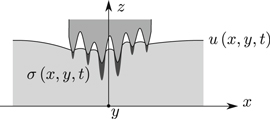
Figure 1. Schematic representation of a rigid punch indenting a viscoelastic half-space. Here,  is the normal displacement of the rigid surface and
  the normal contact stress at time t.
Download figure:
Standard image High-resolution imageThe contact mechanical problem, at time t, is governed by the following boundary conditions at the surface:
where  is the indentation depth, h(x, y) the surface of the rigid punch and
  the region in contact. Moreover, there is no externally applied shear traction so the only tangential traction is caused by the viscoelastic nature of the body.
The differential constitutive equation of a generic viscoelastic material at a given temperature reads

where σ(t) and  (t) are the stress and strain history tensor, and
  are the material constants [46]. Decomposing the stress and strain history tensors in a hydrostatic
  and deviatoric
  part one can write

The four sums over the material constants are often expressed through symbolic operators PK(t), QK(t), PG(t), QG(t) of the type

Here we assume that our viscoelastic material is elastic in dilatation and is described in shear by the Zener model [46]. The time-dependent shear modulus  is defined by the Prony series expansion as

The instantaneous shear modulus  , the adiabatic shear modulus Gt→∞, the relaxation time
  and the retardation time
  are:
are:

where G0 and G1 are the shear moduli and η the viscosity in the Zener model [46]. Combining equations (3)–(5), allows us to give the material constants as:
where K is the bulk modulus. Therefore, equation (3) takes the form:

The rheological representation of the Zener model is given for reference in figure 2.
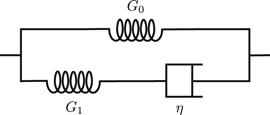
Figure 2. Rheological representation of the Zener model with shear moduli G0 and G1, and viscosity η.
Download figure:
Standard image High-resolution imageIn Laplace space the equivalence between integral and differential expression of the constitutive relation allows one to relate the shear and bulk moduli to the symbolic operators as follows:

where the Laplace transform  of
of  is indicated by the over-bar, with s the complex frequency.
  and
and  have the same coefficients as the material constants in equation (3). For the Zener model
  is:
is:

3. Solution through GFMD
In the GFMD technique, the surface of the deformable solid is discretized with nx × nx equi-spaced grid points that interact with each other through an effective stiffness [35]. When the grid points are displaced by the indenter to a new configuration, the static elastic solution to the boundary value problem is obtained numerically in reciprocal space through damped dynamics [35, 36, 47]. The advantage of working in reciprocal space is that the stiffness matrix is symmetric and diagonal [41], so that each mode can be damped independently. For an elastic solid the areal elastic energy reads [47]:

where  is the Fourier transform of
  , with wave vector
  . As usual,
  is the effective modulus with E the elastic modulus and ν the Poisson's ratio. The elastic normal stress corresponding to the wave vector
  at time t is

Instead of an elastic material we here consider a solid elastic in dilatation and viscoelastic in shear. One can substitute E* in equation (12) with the corresponding expression in terms of shear modulus G(t) and bulk modulus K,

We further assume that the solid is incompressible, so that  , and therefore:

In virtue of the extended elastic–viscoelastic correspondence principle [48], we can find the solution to our viscoelastic boundary value problem relating the analytical Laplace transform of equation (14) and  in equation (10) as follows:

Substituting equation (7) of the Zener model in equation (15), taking the analytical inverse Laplace transform, and assuming that stress and displacement vanish for t ≤ 0, we write the differential formulation for a given wave vector  at time t as

To use a more compact notation, we define C1,2,3,4 as the coefficient to the stress  and displacement
  , obtaining:

with C1 = 1 for the Zener model. The exact numerical integral solution of equation (17) requires the storage of the whole history of stresses and displacements and therefore becomes, with time, progressively more demanding in terms of memory and computational time. To reduce the computational effort, we opt for integrating the equation using the SA method. In the SA method, the simulation time is divided into n equal time periods of duration Δt over which equation (17) is integrated exactly, while the displacement rate is assumed to be constant [44, 49]. The stress in equation (17) can then be expressed as:
where dτ is the differential of time t,

The integration scheme for a given wave vector  is
is
When numerically evaluating the exponents on the right-hand side of equation (20), we use the Taylor-series expansion of the oth-order to prevent numerical rounding errors for small Δt/C2.
The advantage of this method over exact numerical integration is that one only has to save the displacement  and stress
  across time-steps, contrary to saving the whole history of stresses and displacements. An alternative method to save computational resources is the backwards Euler process [44]. Our preference goes to the SA method because it has a second-order and up local error, where the backward Euler method has a zeroth-order and up error for the same Δt, as long as
  [44]. The local error is defined as the difference over a given time-step Δt between the Taylor-series expansions of the exact and integrated analytical solution. Note that the computational time required for the SA method is negligibly different from that required for the backward Euler method, since the only time difference is given by the one-time evaluation of the Taylor-series expansion.
The quasi-static solution at time  is obtained by solving the equation of motion for each mode with a unit mass in reciprocal space over a dimensionless time-step Δt* via the position (Störmer-)Verlet (pSV) algorithm [50]. Note that the dimensionless time-step Δt* is a numerical operator without any physical meaning while Δt has the dimension of time. The quasi-static solution is found quickest by critically damping each mode in reciprocal space. Hereby, we prevent overdamping the equation of motion through a non-monotonous adiabatic critical damping coefficient:

In the limit  , the critical damping coefficient for the pSV is equivalent to that of an harmonic oscillator. When the a priori calculated dimensionless equilibrium time
  is reached, the stresses and displacements in reciprocal space are saved as input for the next dimensional time-step. A hard-wall boundary condition is applied in real space to prevent inter-penetration at the interface. The pseudo-code used to obtain the numerical results is presented in the appendix.
4. Numerical results: indentation by a rigid smooth cylinder
In this section, we aim at validating the newly developed viscoelastic GFMD method through comparison with results obtained using the commercial finite-element software ABAQUS [45]. Note that the finite element method is well suited to study the contact response of smooth bodies in contact, while for rough surfaces, where many discretization points are needed, the GFMD technique is computationally more efficient.
Simulations are performed in two-dimensions for a rigid smooth cylinder of radius  , where
  is the periodic width of the simulation unit cell. The parabolic profile of the cylinder is

where ρ is the distance from the vertical axis of symmetry.
The rigid indenter displaces as follows:
where the load h0 is defined as  . The maximum indentation depth is
  , in the small strain regime. In figure 3, we give the schematic representation of the case studied here.
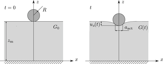
Figure 3. Schematic representation of the initial configuration and indentation by the rigid smooth cylinder to indentation depth  and contact area
  .
.
Download figure:
Standard image High-resolution imageThe viscoelastic solid is taken to have height zm large enough so that we can approximate its response as that of a semi-infinite solid. The average normal displacement of the surface um is

where  is the mean contact pressure [51]. For the incompressible solids in this work the average displacement of the surface um is zero. Therefore, the GFMD simulations are performed assuming that the center-of-mass mode does not move. The surfaces in the GFMD simulations are discretized with
  equi-spaced grid points. The FEM simulations are performed, instead, for a finite sized unit cell of height
  , periodic in x-direction. The boundary of the square
  domain is discretized at the top with 213 equi-spaced nodes. The elements are irregular quadrilaterals and their shape and aspect ratio changes gradually depending on the region they discretize. In the region where the stress gradients are expected to be large the mesh is very fine and comprises elements with aspect ratio close to one. This zone has
  width at the top, where amax is the contact area at maximum indentation depth, and has the same maximum depth, with a parabolic shape at its lower boundary. From there, the size of the elements increases gradually and reaches a larger aspect ratio at the bottom where the stress is homogeneous. The borders of the unit cell are discretized with 29 nodes, the bottom with 27 nodes.
The instantaneous shear modulus  is from now on indicated as
  and the adiabatic shear modulus Gt→∞ as G0 according to their respective frequency response. The ratio between instantaneous and long-time response to a step-load,
  is taken to be 10, unless otherwise specified and the relaxation time Tz = 0.01 s. Time in GFMD is discretized using
  . This is sufficient to ensure convergence of the results. The isotropic rate-dependent material behavior in ABAQUS is described through the small-strain time domain viscoelastic material model (see [45]). The viscoelastic material is defined by a Prony series expansion of the dimensionless relaxation modulus, where the strain components are interpreted as state variables that control the stress relaxation. An a priori user-defined 0.001 strain error tolerance across dimensional time-steps is given [45, 46].
The change in relative contact area, defined as  , and the reduced pressure
  , where
  is the root mean square gradient over the contact area aact, are reported in figures 4(a) and (b) as a function of time for the loads h0 = 0.005, 0.01, 0.02 and 0.05. A good correspondence between the GFMD and FEM results is observed for loads up to h0 = 0.02. For larger loads the discrepancy is given by the fact that the FEM unit cell has a large but finite height. When the cylinder is held constant for t ≤ Tz the contact area becomes constant while the pressure decreases up to t/Tz ≈ 6. At the hold the contact area does not change. This is in line with the analytical solution provided by Christensen [10] for the indentation by a rigid Hertzian.
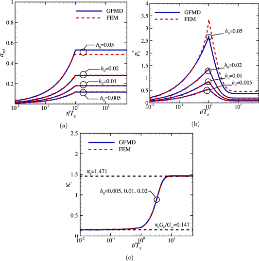
Figure 4. (a) The relative contact area  , (b) the reduced pressure
  , and (c) the proportionality coefficient
  as a function of the normalized time t/Tz for the loads h0 = 0.005, 0.01, 0.02, 0.05.
Download figure:
Standard image High-resolution imageFigure 4(c) shows the proportionality coefficient  as a function of the normalized time t/Tz for the three loads for which there is agreement between FEM and GFMD. The figure contains also the analytical values for the limiting cases of the instantaneous and steady-state proportionality coefficients,
  [52] and κr = 1.471, which show good correspondence with the numerical results. The method is thus validated for both its adiabatic and transient response.
4.1. Numerical results: rolling of a rigid cylinder
The second problem we will consider is the frictionless rolling of a rigid cylinder on a semi-infinite incompressible viscoelastic solid, as depicted in figure 5. The steady-state analytical solution with which our results are compared was provided by Hunter [18]. The transient response is here given for the first time.

Figure 5. Schematic representation of the initial contact and subsequent rolling of the rigid smooth cylinder with tangential velocity  .
.
Download figure:
Standard image High-resolution imageA far-field normal load,

is applied such as to ensure a relative adiabatic contact area arel = a0/R = 1/4. The radius  is selected to ensure no interaction between neighboring indenters. During rolling, the viscoelastic semi-infinite body experiences a displacing normal load but no tangential tractions, given that the interface is frictionless. However, due to the viscoelastic nature of the material, the displacements and the stress fields at any given moment depend on the tangential velocity
  . Therefore, a time-dependent tangential load Lt resists the frictionless sliding of the indenter. The tangential load is inferred from the local load balance as

where aact is the contact area. The dissipative friction coefficient μ is defined as the ratio between the tangential and normal loads, i.e.  . Note that here friction is only intended as the viscoelastic resistance of the bulk. Following Hunter [18], the normalized friction coefficient
  can be expressed as a function of the dimensionless velocity
  . Furthermore, we choose similarly to Hunter [18] the shear moduli
  and prescribe the velocity
  , where H(t) is the Heaviside step-function.
In figure 6(a), the scaled steady-state normal load L/L0 is presented as a function of x/a0 for a cylinder moving with velocity  on viscoelastic half-planes with constants
  . Here, L is the normal load on the surface at a given x-position and L0 is the adiabatic Hertzian normal load at x-position ρ = 0. The shear modulus ratio
  corresponds to the adiabatic case, i.e. no viscous dissipation. The rolling direction is indicated by the black arrow pointing to the right.
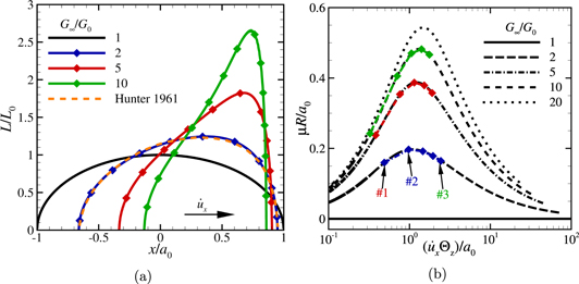
Figure 6. (a) The scaled steady-state normal load L/L0 as a function of the normalized x-position x/a0 with  for
for  and the analytical result by Hunter 1961 [18] for
  . (b) Steady-state normalized friction coefficient μR/a0 as a function of the dimensionless velocity
  for various
  . The black (dashed) lines are the analytical results by Hunter [18], the colored diamonds are numerical results and the colored dashed lines are guides to the eye.
Download figure:
Standard image High-resolution imageThe eccentricity of the load profile is found to increase with increasing  , so does the maximum value of the normal load. The results are in agreement with the analytical solution of Hunter 1961 [18], shown in figure 6(a) for
  .
.
Notice that for the simulations just presented the contact area is not ever increasing with time, which is a necessary condition to invoke the elastic–viscoelastic correspondence principle that we used in section 3. The solution presented in section 3 can, however, also be obtained through the Boussinesq's equation in [43], which does not have the requirement of an ever increasing contact area, and can therefore be used also here.
In figure 6(b), the normalized friction coefficient μR/a0 is shown as a function of the dimensionless velocity  . We observe good correspondence between all numerical results (colored diamonds) and the analytical result (black lines) by Hunter [18]. In line with the results in figure 6(a), the dissipative friction increases with increasing
  . Furthermore, as expected [18, 24], the maximum dissipative friction is attained for
  , see for instance the point indicated with No.
  for
for  . The other two points indicated on the same curve have the same friction coefficient at steady-state, but their transient dissipation is far from similar. This can be seen in figure 7(a), where μR/a0 is given as a function of t/Θz for the rolling velocities
  corresponding to the points Nos.
  ,
,  and
and  in figure 6(b). Constant dissipative friction coefficients are achieved after t/Θz ≈ 5. These are the steady-state values in figure 6(b). By increasing velocity
  from
from  to
to  the maximum transient dissipative friction μmax increases and the time t/Θz at which the maximum is observed, decreases.
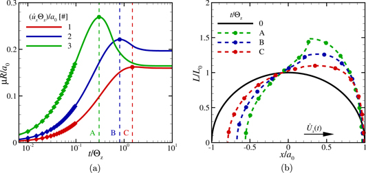
Figure 7. (a) Normalized friction coefficient μR/a0 as a function of t/Θz with  and
and  indicated in figure 6(b) by Nos.
  ,
,  and
and  . The data points are shown with colored diamonds only up to t/Θz = 0.1 for clarity. (b) The scaled normal load L/L0 as a function of x/a0 for t/Θz indicated in (a) by
  ,
,  and
and  .
.
Download figure:
Standard image High-resolution imageIn figure 7(b) the loads L/L0 corresponding to the maximum transient dissipative friction μmax, indicated in figure 7(a) by colored circles, are presented as a function of x/a0. The maximum normal load on the surface as well as the eccentricity of the load profile  increase with increasing velocity
  (from
(from  to
to  ). This agrees once more with the increase in the maximum transient dissipative friction μmax from the normalized time
  to
to  and down to normalized time
  in figure 7(a).
For all rolling velocities and shear moduli studied here it is found that: (1) The maximum transient dissipative friction coefficient μmax increases with velocity  for all shear moduli
  (2) The maximum transient dissipative friction coefficient μmax is larger than the steady-state friction coefficient for all velocities
  studied. The maximum observed in the transient friction coefficient μmax corresponds to the stiction spike observed in the analytical work presented by Persson and Volokitin [21] and in the simulations of Bugnicourt et al [43]. The maximum is caused by the sudden increase in rolling velocity at time t = 0, and is largest for the largest initial velocity step. A similar increase in the static friction coefficient, although in the presence of adhesion at the surface, was measured in the experiments of Roberts and Thomas [53]. In their work, soft polymers show a large increase in friction coefficient compared to hard polymers. The authors observed a strong contribution of viscoelasticity to the overall frictional response for soft polymers. In our work, since the interface is frictionless, the only contribution to friction is provided by the viscoelastic response of the half-plane.
5. Concluding remarks
There is the need for efficient computational techniques to model multi-length-scale roughness and viscoelasticity while accounting for interfacial interactions. As a first step in this direction, we derive the Green's function for a quasi-static incompressible isothermal viscoelastic half-space. We implement the SA method as time-integration scheme [44] to obtain a fast and accurate solution of the equations of motion. The extension to the GFMD method provided in this work allows one to predict the transient and steady-state response of frictionless contacts.
The model is here applied to study the frictionless indentation and rolling of a smooth infinitely long rigid cylinder on a viscoelastic half-plane. These simple problems provide the means of validating the new method through comparison with results obtained by the finite element method and Hunter's analytical work. Additionally, the transient response upon rolling of the cylinder is here given for the first time.
The GFMD method presented and validated in this work provides a platform to model adhesional contacts in future work. This is needed as most interesting phenomena are related to the transient response under reciprocating mixed-mode loading of adhesive contacts, e.g. peeling of pressure sensitive adhesives.
Acknowledgments
LN acknowledges funding from the European Research Council (ERC) under the European Union's Horizon 2020 research and innovation programme (Grant Agreement No. 681813).
: Appendix. Viscoelastic GFMD pseudo-code
- (i)Setup rigid indenter with initial surface topography

- (ii)Determine damping coefficient such that all modes are critically damped and calculate the dimensionless equilibrium time for a given dimensionless time-step
- (iii)Loop over n iterations with time-step until is reached. Give the location of the rigid indenter as , where and are the normal and tangential displacement of the indenter at time .
- (a)Loop over until the dimensionless equilibrium time is reached;
- 1.Discrete fast Fourier transform (DFFT) surface displacement using the FFTW3 library [54];
- 2.Calculate viscoelastic restoring force:
- 3.Add external force and interfacial force, ;
- 4.Add damping forces,
- 5.Use pSV to solve equation of motion,
- 6.Assign and
- 7.Reverse DFFT displacement into real space, and scale displacement with
- 8.Implement the hard-wall
- 9.Calculate interfacial force and DFFT to .
- (b)DFFT displacement
- (c)Save and .


