

Abstract
Objective. To investigate similarities and differences in the formalism, processing, and the results of relative biological effectiveness (RBE) calculations with a biological weighting function (BWF), the microdosimetric kinetic model (MKM) and subsequent modifications (non-Poisson MKM, modified MKM). This includes: (a) the extension of the V79-RBE10% BWF to model the RBE for other clonogenic survival levels; (b) a novel implementation of MKMs as weighting functions; (c) a benchmark against Chinese Hamster lung fibroblast (V79) in vitro data; (d) a study on the effect of pre- or post- processing the average biophysical quantities used for the RBE calculations; (e) a possible modification of the modified MKM parameters to improve the model accuracy at high linear energy transfer (LET). Methodology. Lineal energy spectra were simulated for two spherical targets (diameter = 0.464 or 1.0 μm) using PHITS for 1H, 4He, 12C, 20Ne, 40Ar, 56Fe and 132Xe ions. The results of the in silico calculations were compared with published in vitro data. Main results. All models appear to underestimate the RBEα of hydrogen ions. All MKMs generally overestimate the RBE50%, RBE10% and RBE1% for ions with an LET greater than ∼200 keV μm−1. This overestimation is greater for small surviving fractions and is likely due to the assumption of a radiation-independent quadratic term of clonogenic survival (ß). The overall RBE trends seem to be best described by the novel 'post-processing average' implementation of the non-Poisson MKM. In case of calculations with the non-Poisson MKM, pre- or post- processing the average biophysical quantities affects the computed RBE values significantly. Significance. This study presents a systematic analysis of the formalism and results of widely used microdosimetric models of clonogenic survival for ions relevant for cancer particle therapy and space radiation protection. Points for improvements were highlighted and will contribute to the development of upgraded biophysical models.
Export citation and abstract BibTeX RIS
Abbreviations
| α | linear term of the linear-quadratic model of clonogenic survival |
| ß | quadratic term of the linear-quadratic model of clonogenic survival |
| BWF | biological weighting function |
| DNA | deoxyribonucleic acid |
| LET | linear energy transfer |
| IAEA | International Atomic Energy Agency |
| ICRU | International Commission on Radiation Units and Measurements |
| LQM | linear-quadratic model of clonogenic survival |
| MKM | microdosimetric kinetic model (Hawkins 1994) |
| modified MKM | modified MKM (Kase et al 2006) |
| non-PoissonMKM | corrected version of the original MKM to account for the non-Poisson distribution of lethal lesions (Hawkins 2003) |
| PHITS | Particle and Heavy Ion Transport code System (Sato et al 2018) |
| PIDE | Particle Irradiation Data Ensemble (Friedrich et al 2013) |
| RBE | relative biological effectiveness |
| RBES | in vitro clonogenic cell survival RBE for the surviving fraction S |
| SOBP | spread out Bragg peak |
| V79 | Chinese hamster lung fibroblasts |
| V79-RBE10% BWF | biological weighting function from Parisi et al 2020b |
1. Introduction
The number of clinical centers offering cancer radiation therapy with ions, mostly protons (Paganetti et al 2021) and carbon ions (Malouff et al 2020), is rapidly increasing worldwide because of the superior physical (improved dose conformity, Durante and Paganetti 2016) and biological properties (higher biological effectiveness, Tommasino and Durante 2015, Tinganelli and Durante 2020) of the treatment with respect to the X-rays of conventional radiotherapy. In this regard, it is well known that the radiation-induced damage in living organisms is strongly affected by the exposure characteristics (i.e. dose, dose rate, particle type, LET, fractionation), the system's ability to react to the stimulation, and the biological endpoint considered (Scholz 2003, McMahon and Prise 2021). Therefore, the relative biological effectiveness (RBE, IAEA 2008) of the radiation and its changes over the irradiated volume must be considered while planning a radiotherapy treatment with charged particles. Neglecting these RBE changes might result in zones of unwanted under- or over- dosage and suboptimal treatment outcomes (Wedenberg and Toma‐Dasu 2014, Peeler et al 2016, Wang et al 2020).
Because of its relevance for clinical tumor control probability (TCP) calculations (Fertil and Malaise 1985, Warkentin et al 2004, Paganetti 2017), the in vitro clonogenic survival is one of the most studied biological endpoints. Consequently, RBE calculations based on the clonogenic survival assay are used in clinics for treatment planning purposes (Kanai et al 1999, Inaniwa et al 2010, Mairani et al 2013). The clonogenic survival data (the surviving fraction S as a function of the absorbed dose D) is generally fitted with the linear-quadratic model (LQM, equation (1), Fowler 1989, McMahon 2018):

where α and ß are exposure- and cell- specific radiosensitivity parameters representing the number of lethal events per cell per unit of dose or dose squared respectively (Jones and Dale 2018).
Although there is general consensus in literature on the ion-specific LET-dependence of α, the behavior of ß as function of the LET is topic of discussion, with different models and experiments showing contrasting results (Stewart et al 2018). Nonetheless, the linear term of the LQM for repair competent cell lines is generally characterized by an ion-specific increase with the increase LET up to 100–200 keV μm−1. At higher LET values, α decreases due to overkill effects (Friedrich et al 2013). In case of repair deficient cell lines, the increase in α appears to be significantly lower than for repair competent cell lines (McMahon et al 2017). On the other hand, despite that a vanishing ß is generally observed for exposures to high LET ions, no clear trend in the LET-dependence of ß is present for energetic ions (Furusawa et al 2000, Friedrich et al 2013). This uncertainty is due to the large dispersion of the biological data (Friedrich et al 2013, Parisi et al 2021), the apparent dose-dependence of ß associated to the transition of the survival curve to a constant slope at high doses (Fowler 1989, Astrahan 2008, Park et al 2008, Matsumoto et al 2019) and possible dose-rate effects (Brenner et al 1998, Matsuya et al 2018). Nonetheless, many approaches relying on the LQM formalism were developed and used for in silico computation of the clonogenic survival (Stewart et al 2018, Bellinzona et al 2021).
It is generally accepted that predictive models dealing with systems characterized by sensitive targets in the order of micro- and nano- meters (i.e. DNA, chromatin loops) must take into account the stochastic behavior of the energy deposition at these scales. The study of the stochastic nature of the energy deposition is referred to as microdosimetry (ICRU 1983) and was developed in the 1950s to overcome the limits of average quantities such as absorbed dose and the linear energy transfer (LET) in describing the radiation effects on biological samples.
Two main approaches are used for calculating the RBE using microdosimetric distributions: the ones based on the microdosimetric kinetic model (MKM, i.e. Hawkins 1994 Hawkins 2003, Kase et al 2006, Sato and Furusawa 2012), and the biological weighting functions (BWF, i.e. Morstin et al 1989, Loncol et al 1994, Parisi et al 2020b). Microdosimetric models have the advantage of dealing with quantities such as the specific energy and the lineal energy, which are experimentally measurable (Rossi and Zaider 1996, Lindborg and Waker 2017). Alternatively, approaches based on amorphous track structure calculations could be used (Katz et al 1971), such as the clinically-implemented Local Effect Model (Scholz and Kraft 1994, Elsässer et al 2010). In such models, the clonogenic survival RBE is calculated by coupling the simulated radial dose distribution around the ion track with the experimentally-determined biological dose-response after photon exposures. Furthermore, models based on different assumptions were also proposed, such as particle-specific phenomenological RBE-versus-LET correlations (Kanai et al 1999, Jones et al 2015, Rørvik et al 2018), the repair-misrepair-fixation model (RMF, Carlson et al 2008), the giant loop binary lesion model (GLOBE, Friedrich et al 2012), the biophysical analysis of cell death and chromosome aberrations model (BIANCA, Carante et al 2018), nanodosimetric models (Villegas et al 2016, Conte et al 2018, Schneider et al 2020), the multi scale approach (MSA, Surdutovich and Solov'yov 2019), and the mechanistic DNA repair and survival model (Medras, McMahon et al 2021). Finally, it is worth mentioning that the RBE relative to endpoints other than the clonogenic survival can also be modelled. As an example, the yield of DNA damages and their clustering was computed using different approaches based on track structure codes such as KURBUC (Nikjoo et al 2016), PARTRAC (Friedland et al 2017), GEANT4-DNA (Kyriakou et al 2022), RITRACKS (Plante et al 2013), and PHITS (Matsuya et al 2020).
This work aims to explore the similarities and differences in the formalism and results of the original MKM (Hawkins 1994), the non-Poisson MKM (Hawkins 2003), the modified MKM (Kase et al 2006) and the BWF from Parisi et al (2020b). Since the BWF from Parisi et al (2020b) was developed to phenomenologically reproduce only the RBE relative to a surviving fraction of 10% (RBE10%), this article introduces a methodology to calculate the linear term of the LQM (α) from the results of this BWF and therefore compute the RBE relative to any arbitrary surviving fractions.
In vitro data for the most used mammalian cell line (Chinese hamster lung fibroblasts, V79) were extracted from the Particle Irradiation Data Ensemble (PIDE, Friedrich et al 2013) and used to benchmark the results of the different models.
Additionally, most of the models mentioned above are based on average biophysical quantities (i.e. the dose-mean lineal energy) that are related to the biological effects (i.e. α) through linear or nonlinear relationships. The effect of pre- or post- processing the average physical quantities during the RBE calculations is also investigated.
2. Methodology
2.1. Microdosimetry
In this article, the following definitions apply as defined in ICRU (1983, 2011).
The lineal energy y is a stochastic quantity defined as the quotient between the energy imparted ε by a single event in a given volume of matter and the mean chord length  of that volume. The mean chord length of a volume is the mean length of randomly oriented chords through that volume. For a spherical volume, the mean chord length is equal to 2/3 of the diameter.
The non-stochastic dose-mean lineal energy  is calculated as in equation (2):

where d(y) is the dose probability density d(y) of the lineal energy y.
2.2. Computer simulations
All calculations were performed using the Particle and Heavy Ion Transport code System (PHITS, Sato et al 2018) following the methodology described in previous works (Parisi et al 2021, 2020b). Monoenergetic beams of 1H, 4He, 12C, 20Ne, 40Ar, 56Fe and 132Xe ions of energy equal to 1, 2, 3, 4, 5, 6, 7, 8, 9, 10, 20, 30, 40, 50, 60, 70, 80, 90, 100, 200, 300, 400, 500, 600, 700, 800, 900, 1000 MeV n−1 were simulated. These ions were chosen for their relevance for particle therapy and radiation protection in space, and because these are the ions for which most in vitro data is available.
Both the microdosimetric spectra and the LET were calculated over an infinitesimal layer of water using the PHITS [T-SED] and [T-LET] tallies (PHITS manual, https://phits.jaea.go.jp/manual/manualE-phits.pdf). This was done to efficiently tackle the large variability of the experimental setups used for the in vitro data of paragraph 2.4, and to generate particle-dependent LET-trends which could be used in combination with simulated LET spectra in more realistic scenarios. The secondary electrons produced by the ions (δ-rays) were not transported to avoid double counting their contribution to the microdosimetric spectra (PHITS manual, https://phits.jaea.go.jp/manual/manualE-phits.pdf).
The microdosimetric function (Sato et al 2006, 2012) implemented in the [T-SED] tally of PHITS was used to analytically calculate the microdosimetric spectra. The function can quickly compute microdosimetric distributions in spherical targets (diameter between 1 and 2000 nm) randomly placed around the particle track. The input parameters of the PHITS microdosimetric function are the particle charge, its energy, the LET and the target diameter. The diameter of the spherical water targets (density = 1 g cm−3) was set to 0.464 μm and 1 μm as required by the formalism of the modified MKM and the V79-RBE10% BWF respectively. More details on the PHITS microdosimetric function can be found in Sato et al (2006, 2012).
A logarithmic binning from 10–2 to 107 keV µm−1 with 50 bins per decade was used to score the lineal energy for all particle-target size combinations. In agreement with previous models of radiation-action for luminescent detectors (Parisi et al 2018) and cells (Parisi et al 2020b), the minimum energy deposition considered in the microdosimetric calculations was the one relative to one event of one ionization only (10.9 eV, Sato et al 2006). This corresponds to a lineal energy of approximately 0.035 keV μm−1 and 0.016 keV μm−1 for spherical water targets with diameter equal to 0.464 μm (MKMs) and 1 μm (BWF) respectively.
The unrestricted LET in water values, needed for both the calculations with the PHITS microdosimetric function and to facilitate the comparison between the in silico calculations and the corresponding in vitro data, were determined with the ATIMA model (http://web-docs.gsi.de/∼weick/atima) implemented in the [T-LET] tally of PHITS. Because of the infinitesimal target considered for the LET calculations, the particle slowing down was negligeable; therefore, track- and dose- mean LET values were equivalent.
The experimental exposures were performed with quasi-monoenergetic beams due to the nature of accelerated beams and the presence of material upstream the irradiated cells (i.e. scatterers, energy degraders, cell flask walls...). This can cause some differences in the calculated average LET values. Likewise, the inclusion of the secondary fragments in the calculation of the average LET and the use of different approaches (stopping power tables, different LET models) significantly influence the LET results. The in vitro data included in this study (paragraph 2.4) were extracted from published studies in which different LET methodologies for the calculation were used. Furthermore, details on the LET calculations were not always reported. In some cases, the LET values were not explicitly mentioned and were calculated a posteriori (Friedrich et al 2013). Therefore, it was decided to not indicate the LET average methodology when performing a comparison between in silico and in vitro data. In other words, all results included in this study are plotted as a function of a generic 'unrestricted LET in water'.
Finally, during the calculations encompassed in this study, a limitation in the PHITS microdosimetric function was discovered: the microdosimetric spectra calculated by the function for ions heavier than 20Ne with an energy lower 10 MeV n−1 have an inappropriate peak due to the simple interpolation of the parameters used in the model. A revised version of the PHITS microdosimetric is under development (personal communication with Tatsuhiko Sato, PHITS team leader) starting from the results of track structure simulations obtained with novel PHITS track structure models (Ogawa et al 2021). Consequently, the results of these low-energy heavy-ions were not included in this article. Nonetheless, this has no effect on the conclusions encompassed in this study.
2.3. Biophysical models
This section briefly describes the models used for the clonogenic survival calculations. It is worth noting that all models correlate the in vitro cell death to radiation-induced damaging events within domains located within the cell nucleus. These domains are generally modelled using simulated water spheres with a diameter of approximally 0.5–1 μm (Hawkins 1994, 2003, Kase et al 2006, Sato et al 2011, Sato and Furusawa 2012, Parisi et al 2020b). These spheres are meant to be representative of cellular structures such as giant chromatin loops or chromosome territories (Kellerer and Rossi 1978, Yokota et al 1995, Meaburn and Misteli 2007, Friedrich et al 2012). The inactivation of one of these domains is assumed to lead to cell death. Other in vitro mechanisms of cells death such as membrane rupture or intracellular communication (bystander effects) are not accounted in this study. Similarly, because of the large spread in the data and the uncomplete report of dosimetric information in most publications (Parisi et al 2021), dose rate effects are not explicitly considered.
The following models were considered in this article: the original MKM (Hawkins 1994), the non-Poisson MKM (Hawkins 1994), the modified MKM (Kase et al 2006) and the biological weighting function from Parisi et al (2020b). In all cases, the following quantities were assessed and compared with corresponding in vitro data (paragraph 2.4): RBEα , RBE50%, RBE10%, RBE1%.
The RBE for the linear term of the LQM (RBEα ) was defined as in equation (3) as the ratio between the corresponding values after the ion (α) or the reference photon (αref) exposures:

The RBE for the quadratic term of the LQM (RBEß ) was defined as in equation (4) as the ratio between the corresponding values after the ion (ß) or the reference photon (ßref) exposures:

Furthermore, the RBE relative to the surviving fraction S (RBES) was calculated using equation (5) (Parisi et al 2020b):

where α, ß, αref and ßref are respectively the linear and quadratic terms of the LQM for the radiation under investigation and the reference photon exposure.
The expression for RBEα (equation (3)) can be obtained as the limit of RBES (equation (5)) for D→0. On the other hand, the expression for RBEß cannot be derived from equation (5) since the limit of the RBE for D→+∞ tends to the square root of ß/ßref. Because negative values of ß were reported in several in vitro experiments (Friedrich et al 2013), it was decided to define RBEß in this study as the simple ratio between ß and ßref. This was done to facilitate the comparison between in silico and in vitro data, and to not be forced to reject experiments with negative ß values. The negative RBEß values can be due to the presence of a subpopulation of cells with increased radiation resistance (Friedrich et al 2021). Despite the definition of RBEß in equation (4) is quite arbitrary, the calculation of the RBE for an infinite dose as the square root of ß/ßref may be inaccurate since it is well-known that the in vitro clonogenic survival curves at high doses are characterized by a transition to constant slope (Fowler 1989, Astrahan 2008, Park et al 2008, Matsumoto et al 2019). In other words, since ß at high doses appears to be 0, the in vitro RBE for an infinite dose would not be equal to the square root of ß/ßref but to the ratio between the linear terms valid in this dose range (different from α values determined at relatively low doses).
2.3.1. Adaptation of the V79-RBE10% BWF to α
According to the model formalism (equation (6), Parisi et al
2020b), the in vitro clonogenic survival RBE for to a surviving fraction of 10% (RBE10%) can be calculated as the integral between d(y) and the biological weighting function 

ymin is the minimum lineal energy value considered for the RBE calculations and it was set to 0.016 keV μm−1 (lineal energy relative to an event of one ionization only in a 1 μm water sphere, paragraph 2.2).
The BWF is plotted in figure 1 and it is characterized by a flat profile (r(y) ∼ 1) between roughly 0.01 and 1 keV μm−1, a local maximum (r(y) ∼ 4.5) around 130 keV μm−1 and a subsequent decrease is due to overkill effects. The function reaches 0 around 4000 keV μm−1 (ymax).
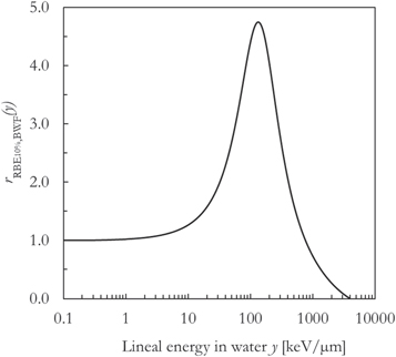
Figure 1. The biological weighting function to calculate the clonogenic survival RBE of the V79 cell line for a surviving fraction of 10%.
Download figure:
Standard image High-resolution imageThis biological weighting function was determined through an iterative process aimed at minimizing the difference between the in silico RBE calculated using PHITS-simulated lineal energy spectra and experimental in vitro RBE10% data points for Chinese hamster lung fibroblasts (V79 cell line) in normoxic asynchronized conditions. The lineal energy spectra were assessed in liquid water for a sphere with diameter equal to 1 μm. Using this unique function, it was possible to reproduce the non-unique LET-dependence of the V79 in vitro RBE10% values for ions from 1H to 238U (unrestricted LET in water range: ∼0.2–15000 keV μm−1) without any adjustments of its shape. In other words, the same BWF can be unchangingly applied to calculate the RBE10% of the V79 cell line for all particles (Parisi et al 2020b).
Recently, it was proven possible to use the V79-RBE10% BWF for modeling in first approximation also the in vitro RBE10% of other repair-competent asynchronized normoxic mammalian cell lines (Parisi et al 2021).
Under the assumption that the quadratic term of the LQM is radiation-independent (ß = ßref as in the original MKM and subsequent modifications,Hawkins 1994, Kase et al 2006, Sato and Furusawa 2012), an expression to calculate α from the results of the BWF was derived (equation (7), see Appendix):

Only positive α values were accepted. The numerical values of αref = 0.184 Gy−1 and ßref = 0.02 Gy−2 were chosen for consistency with the ones used for the calculations with the MKM-based models (see paragraph 2.3.6) Nonetheless, these values are very similar to the ones obtained by averaging the corresponding ones for the V79 photon PIDE entries included in this study, namely αref = 0.189 Gy−1 and ßref = 0.02 Gy−2.
2.3.2. MKM
Following the methodology described in Hawkins (1994), the linear term of the LQM can be assessed using equation (8):

where α0 is a cell-specific constant representing the initial slope of the survival curve in the limit of y → 0, ßref is the quadratic term of the LQM model for the reference photon exposure,  is the dose-mean lineal energy assessed in a domain with density ρ and radius rd. The model parameters are listed in paragraph 2.3.6.
The quadratic term of the LQM was assumed to be radiation independent (ß = ßref). The same assumption holds for the other MKM-based models described in the following paragraphs.
2.3.3. Non-poisson MKM
In a later work (Hawkins 2003), the original model was modified to account for the overkill effects at high LET. An additional factor was introduced in the calculation of α (equation (9)) to consider the non-Poisson distribution of the lethal lesions among the cells:
α0 is the initial slope of the survival curve in the limit of y → 0, ßref is the radiation-independent quadratic term of the LQM model assessed in case of the reference photon exposure,  is the dose-mean lineal energy assessed in a domain (radius rd),
  is the dose-mean lineal energy in the nucleus (radius Rn), and ρ is the density.
For simplicity, it is generally assumed that the dose-mean lineal energy is independent of the site diameter ( Hawkins 2003, Kase et al
2006). Consequently, all lineal energy values included in this article are relative to quantities assessed in the domain.
Hawkins 2003, Kase et al
2006). Consequently, all lineal energy values included in this article are relative to quantities assessed in the domain.
2.3.4. Modified MKM
An alternative way to account for the overkill effects was introduced in Kase et al (2006). In this case, the linear term of the LQM can be assessed using equation (10):

where α0 is the initial slope of the survival curve in the limit of y → 0, ßref is the radiation-independent quadratic term of the LQM model assessed in case of the reference photon exposure,  is the saturation-corrected dose-mean lineal energy assessed in a domain with density ρ and radius rd.
The saturation-corrected dose-mean lineal energy is a phenomenological quantity introduced to reproduce the results of biological experiments (Kellerer and Rossi 1974, Sato et al 2011) and it is calculated using equation (11):

where  is a saturation parameter that can be assessed using equation (12) (Kase et al
2006):
is a saturation parameter that can be assessed using equation (12) (Kase et al
2006):

2.3.5. Implementation of the models as weighting functions
As described in the previous paragraphs, MKMs allow the calculation of the biological effects by analyzing average biophysical quantities such as the dose-mean lineal energy (original MKM and non-Poisson MKM) or the saturation-corrected dose-mean lineal energy (modified MKM). The relationship between these quantities and the biological effect is either linear (original MKM and modified MKM) or nonlinear (non-Poisson MKM). Similarly, the RBE10% calculated with the V79-RBE10% BWF was related to RBEα
through equation (8). In other words, the biological effect is computed as the effect relative to a dose-weighted mean value of the microdosimetric spectrum. Since these models calculate the relevant mean quantities (i.e. 
 ) before computing the resulting biological effect, this article refers to them as 'pre-processing average' models.
Alternatively, we investigate the possibility of calculating α as the dose-weighted mean of the biological effect over each bin of the microdosimetric spectrum. In other words, these 'post-processing average' models firstly calculate the α as a function of the lineal energy for an event of lineal energy y. In a second step, the mean α is calculated by performing a dose-weighted average of the computed α values in each bin.
This process can be mathematically described as in equation (13):

where α(y) is the linear term of the LQM for an event of lineal energy y. ymin and ymax are the minimum and maximum lineal energy values considered for the RBE calculations. The integrations limits depend on the model used (see hereunder).
Similarly, RBEα can be calculated with equation (14):

where the weighting function  was defined as the ratio between α(y) and αref. Equation (14) is equivalent to the one commonly used for RBE calculations with BWFs (Loncol et al
1994, Parisi et al
2020b).
was defined as the ratio between α(y) and αref. Equation (14) is equivalent to the one commonly used for RBE calculations with BWFs (Loncol et al
1994, Parisi et al
2020b).
The weighting functions for the different models were derived by calculating the α value in case of lineal energy spectra composed by an event of lineal energy y. A similar approach was used in Kase et al 2006 while comparing the modified MKM and the non-Poisson MKM.
The  are listed hereunder for the different models.
rRBE α (y) for the V79-RBE10% BWF, equation ( 15 ):

where  is the V79-RBE10% BWF (figure 1, Parisi et al
2020b), ymin = 0.016 keV μm−1 (lineal energy relative to an event of one ionization only in a 1 μm water sphere, paragraph 2.2), ymax = 1100 keV μm−1 (see hereunder).
is the V79-RBE10% BWF (figure 1, Parisi et al
2020b), ymin = 0.016 keV μm−1 (lineal energy relative to an event of one ionization only in a 1 μm water sphere, paragraph 2.2), ymax = 1100 keV μm−1 (see hereunder).
Since only positive values of  were accepted for the calculation of the RBEα
, the weighting function can be used only when the following condition is satisfied (Inequality 16):
were accepted for the calculation of the RBEα
, the weighting function can be used only when the following condition is satisfied (Inequality 16):

namely for  ≥ 0.66 and thus y ≤ ∼1100 keV μm−1.
It is worth noting that the BWF function for RBEα is equal to 0 at ∼1100 keV μm−1, while the BWF for the RBE10% (Parisi et al (2020b) reaches 0 at ∼4000 keV μm−1.
Because of the different upper integration limits (ymax), it is expected that the RBEα assessed using equations (14) and (15) will differ from the one obtained by using the α calculated with equation (7). Consequently, the RBEα was assessed with both methodologies and compared.
rRBE α (y) for the MKM, equation ( 17 ):

ymin = 0.035 keV μm−1 (lineal energy relative to an event of one ionization only in a 0.464 μm water sphere, paragraph 2.2), ymax = +∞ keV μm−1.
The RBEα values calculated with equations (14) and (17) or by using the α from equation (8) were checked to be mathematically equivalent (see Appendix).
rRBE α (y) for the non-Poisson MKM, equation ( 18 ):
ymin = 0.035 keV μm−1 (lineal energy relative to an event of one ionization only in a 0.464 μm water sphere, paragraph 2.2), ymax = +∞ keV μm−1.
Since the relationship between  and α is nonlinear, the RBEα
values calculated using equations (14) and (18) or using the α from equation (9) are expected to differ. Consequently, the RBEα
was assessed with both methodologies and compared.
and α is nonlinear, the RBEα
values calculated using equations (14) and (18) or using the α from equation (9) are expected to differ. Consequently, the RBEα
was assessed with both methodologies and compared.
rRBE α (y) for the modified MKM, equation ( 19 ):

ymin = 0.035 keV μm−1 (lineal energy relative to an event of one ionization only in a 0.464 μm water sphere, paragraph 2.2), ymax = +∞ keV μm−1.
The RBEα values calculated with equations (14) and (19) or by using the α from equation (10) were checked to be mathematically equivalent (see Appendix).
2.3.6. Model parameters
The optimal parameters for the V79 cell line were extracted from Sato et al (2011) and used for the calculations with all MKMs, namely: α0 = 0.105 Gy−1, αref = 0.184 Gy−1, βref = 0.02 Gy−2, rd = 0.232 μm, Rn = 4.14 μm, ρ = 1 g cm−3, and y0 = 133.1 keV μm−1. As stated in paragraph 2.3.1, the same values of αref and βref were used also for the calculations using with the BWF.
The lineal energy spectra were assessed for spherical water targets diameter equal to 0.464 μm and 1 μm as required by the MKMs and the BWF respectively. A comparison between the PHITS-simulated lineal energy distributions for these two targets can be found in Parisi et al (2020b) for different ions and energies.
2.4. In vitro data
2.4.1. PIDE
The experimental in vitro clonogenic survival data needed for the benchmark of the in silico results were extracted from the Particle Irradiation Data Ensemble (PIDE, Friedrich et al 2013) version 3.2 (updated in November 2019, Friedrich et al 2021). The database includes 1118 in vitro clonogenic survival entries for more than 100 cell lines exposed to ions from 1H to 238U. Whenever available, corresponding data for the reference photon exposures are also included. The in vitro data were gathered from 115 papers published between 1966 and 2015. The database encompasses data relative to irradiations of cell lines in normoxic conditions only.
The following physical information are reported in PIDE for each ion exposure: the particle type, its energy, the linear energy transfer (LET) in water, and the type of dose profile used (monoenergetic beam or a spread out Bragg peak). Furthermore, the name of the cell line, its origin (human or rodent), its class (tumor or healthy), and the cell cycle phase are also listed.
All clonogenic survival curves are described using the linear (α) and quadratic (β) terms of the LQM. Two datasets of linear-quadratic terms are included in PIDE: the first reflects the original fit as reported in the original publications included in PIDE, while the second is the result of an automated fit performed by the PIDE team on the raw survival curves. More info can be found in Friedrich et al (2013, 2021).
2.4.2. Data selection
If a PIDE entry reported both sets of linear-quadratic terms (original fit and fit by the PIDE team), double counting was avoided by including the PIDE-fitted linear-quadratic terms only. This was done because the more systematic fit procedure by the PIDE team allows a fairer comparison between the different data sets (Friedrich et al 2021). It was already checked that this choice does not introduce systematic or bias in the data (Parisi et al 2021). In some cases, the PIDE entries do not list complete LQM sets (ion and reference photons) for both fits. Therefore, the results of the two fits were combined, introducing uncertainties whose magnitude is difficult to estimate.
As done in Parisi et al (2021) and for consistency with the monoenergetic computer simulations, in vitro data for experiments using spread out Bragg peaks (SOBPs) were not included. Furthermore, entries for ions with energy < 1 MeV n−1 were discarded to avoid partial cell irradiations and the large uncertainties associated with very-low energy exposures. Because of the influence of the cell phase on the clonogenic survival, only data for asynchronized cell experiments were included in this study.
Corresponding in vitro results for the V79 cell line (Chinese Hamster lung fibroblasts) were used to benchmark the model calculations. It was decided to focus the analysis on the V79 cell line because it is the most used mammalian cell line and represents by far the most abundant fraction of in vitro data in PIDE.
Data from the following ions were included: 1H, 2H, 3He, 4He, 12C, 20Ne, 40Ar, 56Fe and 132Xe ions. Results from different isotopes of the same element (i.e. 1H and 2H) were pooled together since no relevant differences were observed in the obtained RBE-versus-LET trends (Parisi et al 2020b).
2.5. Comparison between data series
In agreement with previous studies (Parisi et al
2021, 2020b), the agreement between the theoretical and the n experimental values was quantified using the average relative difference  (equation (20)) and the average relative absolute deviation
  (equation (21)).
The first quantity  was used to investigate possible systematic under- or ever- estimations between the in silico and in vitro data (not possible to assess using
  ). On the other hand,
  is used as an indication of the average agreement between the data series by preventing that relative difference values of opposite sign would cancel themselves.
Finally, in vitro RBE values equal to 0 were excluded from the calculations with equations (20) and (21):


3. Results
3.1. Comparison between the different RBEα weighting functions
The weighting functions rRBE α(y) derived from the formalism of the V79-RBE10% BWF (equation (15)), the original MKM (equation (17)), the non-Poisson MKM (equation (18)) and the modified MKM (equation (19)) are plotted in figure 2 as a function of the lineal energy in water y.
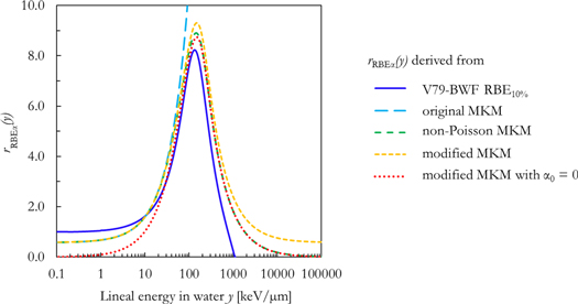
Figure 2. Comparison between the rRBE α (y) functions derived from the V79-RBE10% BWF (equation (15)), the original MKM (equation (17)), the non-Poisson MKM (equation (18)) and the modified MKM (equation (19)) and the modified MKM with α0 = 0 (equation (19), α0 = 0).
Download figure:
Standard image High-resolution imageThe functions are characterized by a reasonable agreement at intermediate lineal energy values (10 < y < 100 keV μm−1). However, relevant differences are present outside this range.
At lower lineal energy values (y < 10 keV μm−1) the functions tend to two different values, namely 1 for the one derived from the V79-RBE10% BWF, and ∼0.57 for the functions based on the MKM. In the first case, this is because the V79-RBE10% BWF was constructed in Parisi et al (2020b) to be ∼1 for y < 1 keV μm−1, in agreement with the corresponding in vitro RBE10% data. On the other hand, the MKM-based rRBE α(y) functions tend to the ratio between α0 and αref (0.105/0.184 = ∼0.57), V79 parameters from Sato et al (2011) for y → 0.
For y > 100 keV μm−1, these differences become even more marked. The rRBE α(y) function based on the original MKM diverges because of its lack of corrections for the overkill effects. By contrast, the other three rRBE α(y) functions show a decrease with the increase of the lineal energy after reaching a local maximum between 100 and 200 keV μm−1. While the rRBEα (y) function derived from the V79-RBE10% BWF reaches 0 at around 1000 keV μm−1, the other two functions (non-Poisson MKM and modified MKM) tend to an asymptotic value of 0 and 0.57 respectively for y → +∞.
Furthermore, a measure of the effect on RBEα induced by an event of lineal energy value y can be obtained by multiplying the rRBE α (y) functions of figure 2 by y 1 . The resulting quantity eRBEα (y) helps visualizing the implementation of saturation effects in the different formalisms (figure 3). It is expected that an e(y) function representing saturation effects would tend to a constant value above a certain threshold of the variable it depends on (in this case, the lineal energy y). Except for the eRBE α(y) function based on the non-Poisson MKM, the other functions behave very differently from the expected saturation behavior. The eRBE α(y) function for the original MKM diverges, the one for the modified MKM shows a monotonic increase after an inflection point, and the function based on the V79-RBE10% BWF sharply decreases reaching 0 around 1000 keV μm−1.
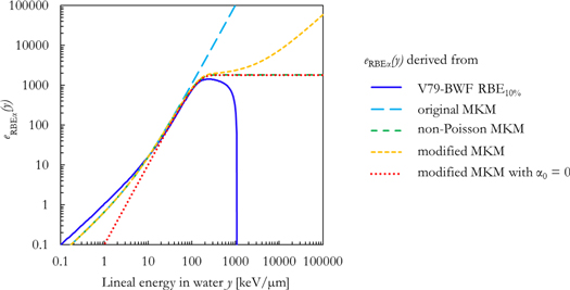
Figure 3. Comparison between the eRBE α (y) functions derived from the V79-RBE10% BWF (equation (15)), the original MKM (equation (17)), the non-Poisson MKM (equation (18)) and the modified MKM (equation (19)) and the modified MKM with α0 = 0 (equation (19), α0 = 0).
Download figure:
Standard image High-resolution imageThe V79-RBE10% BWF was determined in Parisi et al (2020b) to phenomenologically reproduce the V79 in vitro RBE10% data. However, since the in vitro clonogenic survival curves for very high LET exposures (LET > 500 keV μm−1) are characterized by a decrease in both the linear (α) and the quadratic (ß) term of the LQM with respect to the reference photon exposure, the V79-RBE10% BWF intrinsically accounts for the decrease of both terms. In this regard, figure 4 compares the RBEß for the in vitro data included in this study as a function of the LET in water. Despite the large scatter in the in vitro data and an unclear trend for LET < 500 keV μm−1, the RBEß appears to tend to 0 at higher LET values.
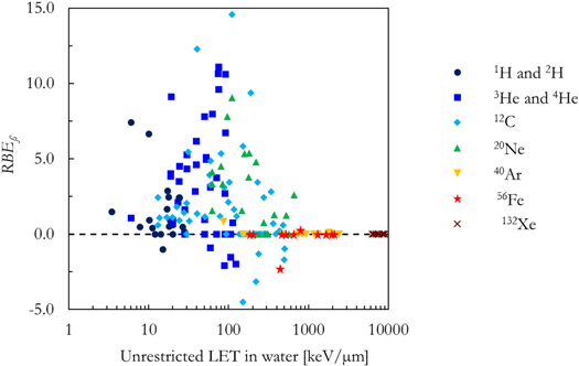
Figure 4. In vitro RBEß for V79 cell line as a function of the unrestricted LET in water for the seven ions included in this article.
Download figure:
Standard image High-resolution imageHowever, in order to derive an expression (equation (7)) to calculate α from the results of the V79-RBE10% BWF, a radiation independent ß was assumed (see Appendix). Consequently, the α values calculated with equation (7) are underestimated at high LET to compensate for the presence of ß = ßref. This causes the sharp decrease of the corresponding weighting functions in figures 2 and 3.
Furthermore, since the increasing behavior of the eRBE α(y) function based on the modified MKM is caused by presence of the constant term α0, an additional weighting function was constructed by setting α0 = 0 in equation (19). The resulting rRBEα (y) and eRBEα (y) functions are also plotted in figures 2 and 3 respectively. This rRBEα (y) is proportional to the saturation-corrected dose-mean lineal energy with no offsets, and therefore the function tends to 0 for y → 0 and for y → +∞ (figure 2). It is worth noting that this rRBEα (y) is very similar to the one for the non-Poisson MKM for y > 200 keV μm−1, i.e. after the local maximum of the functions. Finally, the corresponding eRBEα (y) function (modified MKM with α0 = 0) seems to follow the expected trend for the description of saturation effects (figure 3).
3.2. Benchmark against in vitro data
As a benchmark of the results obtained combining the PHITS-simulated lineal energy spectra (target = water sphere with diameter equal to 0.464 or 1.0 μm) and the different biophysical models, figures 5–8 compare the in silico calculations (RBEα , RBE50%, RBE10%, RBE1%) with corresponding in vitro V79 data from PIDE. The results are plotted as a function of the ion type and the unrestricted LET in water.

Figure 5. Comparison between in silico and in vitro RBEα for seven different ions as a function of the unrestricted LET in water.
Download figure:
Standard image High-resolution image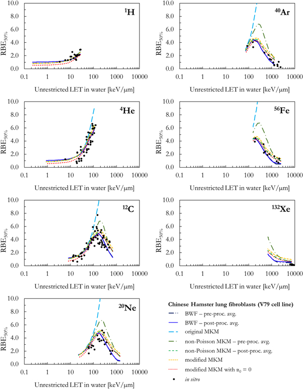
Figure 6. Comparison between in silico and in vitro RBE50% for seven different ions as a function of the unrestricted LET in water.
Download figure:
Standard image High-resolution image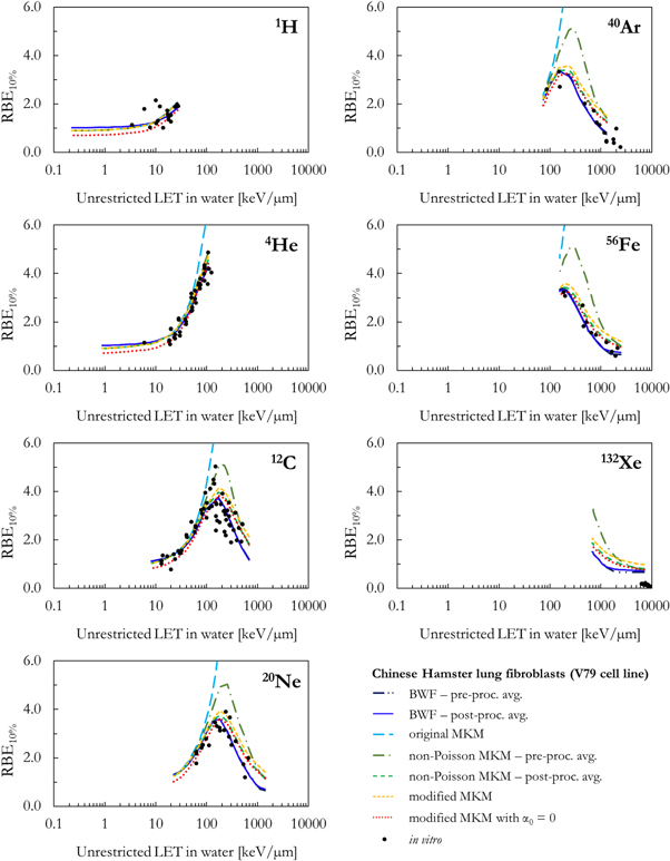
Figure 7. Comparison between in silico and in vitro RBE10% for seven different ions as a function of the unrestricted LET in water.
Download figure:
Standard image High-resolution image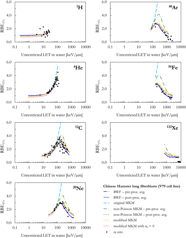
Figure 8. Comparison between in silico and in vitro RBE1% for seven different ions as a function of the unrestricted LET in water.
Download figure:
Standard image High-resolution imageFurthermore, figure 9 shows the average relative difference (equation (20)) and the average relative deviation (equation (21)) as a function of the ion atomic mass number for all biophysical models and RBE endpoints. To facilitate the visualization of the data, the comparison is limited to average relative difference and average relative deviation values up to 2.

Figure 9. Average relative difference (equation (20)) and average relative deviation (equation (21)) between in silico and in vitro RBE values plotted as a function of the atomic mass number of the ion used for the exposures.
Download figure:
Standard image High-resolution image
All RBE data series in figures 5, 6, 7 and 8 follow a similar trend as a function of the LET: the RBE increases with the increase of the LET up to an ion-specific local maximum located around 100–200 keV μm−1. At higher LET values, the RBE decreases due to the well-known overkill effects. Furthermore, smaller RBE values are obtained for RBE values relative to smaller surviving fractions. However, relevant differences are present between the results of the different models.
4. Discussion
In order to fully exploit the potential of cancer radiation therapy with charged particles, accurate and robust biophysical models of radiation induced effects are needed for treatment planning. Because of its relevance of TCP and NTCP, most models consider the clonogenic survival as a relevant endpoint for optimization purposes (Paganetti 2017). However, the clonogenic survival is a complex phenomenon which depends on many factors such as the radiation quality, the dose, the dose- rate, the fractionation scheme, the cellular oxygen level, possible bystander effects, and the chosen cell line (Scholz 2003, Durante et al 2021, McMahon and Prise 2021).
In this work, the effect of radiation quality and dose was systematically investigated by comparing the results of the most used microdosimetric models of clonogenic survival, namely the original MKM (Hawkins 1994), the non-Poisson MKM (Hawkins 2003) and the modified MKM (Kase et al 2006). The BWF from Parisi et al 2020b was also included for comparison and to be representative of modeling approaches based on BWFs. Clonogenic survival in vitro data for the V79 cell line (Chinese hamster lung fibroblasts) were extracted from PIDE (Friedrich et al 2013) and used to benchmark for the model calculations. All results are relative to single-dose exposures in normoxic asynchronized conditions. The V79 cell line was chosen because it is the most used mammalian cell line and represents by far the largest fraction of in vitro data in PIDE. Furthermore, model parameters for cell lines other than the V79 are not always available. The application of selected models to model the RBE of other DNA repair competent or deficient cell lines will be topic of future work.
The MKM (Hawkins 1994) and the non-Poisson MKM (Hawkins 2003) were chosen because they represent the original formulations of the model from which all subsequent MKMs were built. Furthermore, the modified MKM (Kase et al 2006) was included in the comparison because of its clinical relevance (the model has been implemented in particle therapy treatment planning systems in Japan) and its widespread application in combination with simulated or measured microdosimetric spectra (Sato et al 2009, Inaniwa et al 2010, Sato et al 2011, Kase et al 2011a, 2011b, 2013, Inaniwa et al 2015, Takada et al 2017, Debrot et al 2018, Parisi et al 2020a, Bianchi et al 2020, Tran et al 2022). The BWF from Parisi et al 2020b was chosen since it is based on to the same biological endpoint as the MKM models (clonogenic survival). By contrast, the commonly used BWF (Loncol et al 1994) is relative to a different biological endpoint, namely the early intestine tolerance assessed by in vivo crypt regeneration in mice.
Other models such as the stochastic- and double stochastic MKM (SMKM and DSMKM respectively) were proposed (Sato and Furusawa 2012) to overcome the limitations of the modified MKM (Kase et al 2006) in reproducing in vitro data relative to high LET and high dose exposures. However, the SMKM and DSMKM (Sato and Furusawa 2012) strongly differ from the models previously mentioned (Hawkins 1994, Hawkins 2003, Kase et al 2006) since they require the evaluation of dose-dependent microdosimetric distributions, which can be computationally very demanding. Despite that approximate versions of these models were developed to overcome the long computational time and memory requirements (Inaniwa and Kanematsu 2018), the resulting model formalism is based on the description of the clonogenic survival using a cubic polynomial expression in respect to dose. Furthermore, the numerical values of the optimal SMKM and DSMKM parameters (i.e. Rn) generally strongly differ (Sato and Furusawa 2012, Inaniwa and Kanematsu 2018) from the ones for the other MKMs (listed in paragraph 2.3.5). Consequently, a comparison between α and RBE values would be not straightforward. Thus, it was decided to not include the SMKM and DSMKM in the comparison.
Figure 2 shows the original implementation of the MKMs as weighting functions for the calculation of RBEα . This representation helped to understand the differences in the processing of the microdosimetric spectra between the models. It is evident that there are relevant discrepancies between the MKMs, especially at high lineal energy values (the functions tend to different values, namely +∞, 0 or 0.57 for the original MKM, the non-Poisson MKM and the modified MKM respectively). Furthermore, the RBEα weighting function derived from the V79-RBE10% BWF is also included in the same plot. As discussed in paragraph 3.1, the sharp decrease of the function is due to the assumption of a radiation-independent ß. This assumption was necessary to derive equations (7) and (15) and represents a limitation of the current approach. A phenomenological BWF for RBEα could be assessed from the in vitro data as done in Parisi et al (2020b), but it is beyond the scope of this work.
Additionally, a new quantity e(y) (figure 3) was introduced to study the implementation of saturation effects in the different models. It is expected that an e(y) function representing saturation effects would tend to a constant value for y → +∞. This appears to be the case for the non-Poisson MKM. However, things are different for the approaches based on the V79-RBE10% BWF, the original MKM and the modified MKM. In the first case, the sharp decrease in the function is due to the inclusion of the decreasing ß in the model. The e(y) for the original MKM diverges because no overkill corrections are implemented in the model. Furthermore, after reaching an apparent saturation defined by the saturation parameter y0 in equation (19), the effect modelled by the modified MKM increases with the increase of the lineal energy. This is conceptually in contrast with the expected saturation behavior, and it is responsible for the overestimation in the RBEα values calculated with this model at high LET. This increase is due to the presence of the constant term α0 in the model formalism.
To try to mitigate this overestimation, an additional biological weighting function was introduced by setting α0 = 0 in the formalism of the modified MKM. Setting α0 = 0 implies that pairwise combination of lesions is considered the most relevant mechanism of cell death at all dose levels (Hawkins 2005). This function (red dotted line in figure 3) seems to be very similar to the non-Poisson MKM function for y > 200 keV μm−1, and it can adequately describe the saturation effects. Consequently, this version of the modified MKM with α0 = 0 should be regarded as a high LET approximation of the non-Poisson MKM. Nonetheless, at low linear energy (y < 20 keV μm−1) this function seems to be characterized by RBEα values which are too small with respect to the experimental observations (figure 2). As an example, the dose-mean lineal energy for photons generally used as a reference in radiobiological experiments is generally between ∼2 and 4 keV μm−1 (obtained with simple monoenergetic PHITS photon simulations), values in agreement with the ones reported in Kase et al (2006) and Sato et al (2011). The average RBEα calculated by the modified MKM with α0 = 0 ranges between approximately 0.2 and 0.4 for 2 < y < 4 keV μm−1, in contrast with the values as calculated with the other two approaches (∼0.8–1.4). Therefore, an underestimation in the calculated RBEα is expected for low lineal energy particles. This could have been mitigated by multiplying the function by a factor of ∼3. However, this would have resulted in a large overestimation of the RBEα for y > 10 keV μm−1. Consequently, it was decided to use this function without further corrections and to focus the evaluation of its accuracy at high LET.
A systematic comparison between in silico and in vitro RBE data for the V79 cell line can be found in figures 5–8. It seems from figure 5 that all models underestimate the in vitro RBEα for hydrogen ions. The underestimation is the worst for the modified MKMwith α0 = 0. The calculated RBEα values are unreasonably small in case of energetic light particles whose pattern of energy deposition is similar to the one of the reference photons.
Since the original MKM does not include corrections for the overkill effects, the model fails to reproduce all in vitro data relative to exposures to ions with a LET > ∼100 keV μm−1. The ion-specific results of all models are in reasonable agreement with each other and the corresponding in vitro RBEα data for LET < 100 keV μm−1.
For LET > 100 keV μm−1, the in silico RBEα results for the BWF-model, the non-Poisson MKM, the modified MKM and the modified MKM with α0 = 0 differ because of the different implementations of overkill effects (figure 3).
Furthermore, pre- or post- processing the average values during the RBEα
calculations was found to significantly affect the results obtained with the non-Poisson MKM. In this case, the RBEα
values computed by pre-processing  (equation (9)) are significantly higher than the ones obtained with the post-processing approach (equation (18)) in case of 12C and heavier ions. The agreement with the in vitro data is significantly better for the novel post-processing average implementation of the non-Poisson MKM (equation (18)). For the methodology based on the V79-RBE10% BWF, the RBEα
obtained by using both processing methodologies are generally equivalent. However, when the microdosimetric spectra present entries between 1100 and 4000 keV μm−1 (upper integration limits for the equations (15) and (6) respectively), differences were found between the calculated RBEα
values. These differences are most evident for 56Fe and 132Xe ions at relatively low energy. No differences are present between the results of the pre- and post- processing average methods for the MKM and the modified MKM (see Appendix).
(equation (9)) are significantly higher than the ones obtained with the post-processing approach (equation (18)) in case of 12C and heavier ions. The agreement with the in vitro data is significantly better for the novel post-processing average implementation of the non-Poisson MKM (equation (18)). For the methodology based on the V79-RBE10% BWF, the RBEα
obtained by using both processing methodologies are generally equivalent. However, when the microdosimetric spectra present entries between 1100 and 4000 keV μm−1 (upper integration limits for the equations (15) and (6) respectively), differences were found between the calculated RBEα
values. These differences are most evident for 56Fe and 132Xe ions at relatively low energy. No differences are present between the results of the pre- and post- processing average methods for the MKM and the modified MKM (see Appendix).
The overall best agreement with in vitro RBEα data was found for the novel 'post- processing average' non-Poisson MKM.
As a consequence of the similarity between the weighting functions of the non-Poisson MKM and the modified MKM with α0=0 in the high lineal energy region (figures 2 and 3) and the similar RBE results, the modified MKM with α0 = 0 can be considered as a simplified high-LET approximation of the non-Poisson MKM. These findings allow to provide an additional interpretation for the data included in Baiocco et al (2016). In that work, it was found possible to reproduce the energy-dependence of the neutron weighting factors by computing the normalized saturation-corrected dose-mean lineal energy as a function of the incident neutron energy. Remembering that the secondary particles induced by neutrons have generally high LET and that the α calculated using the modified MKM with α0 = 0 is proportional to the saturation-corrected dose-mean only, the energy dependence of the neutron weighting factors (valid for low dose) can be explained as the evolution of the corresponding α (LQM term dominant at low dose) as a function of the neutron energy as calculated with the modified MKM with α0 = 0.
On the other hand, the results of the BWF and the modified MKM are respectively under- and overestimating the in vitro RBEα . This is particularly evident for 56Fe and 132Xe ions.
Differently from what obtained in case of RBEα , the in silico proton RBE50% values (figure 6) are in reasonable agreement with the corresponding in vitro data. For the other ions, the discussion of the RBE50% results is similar to the one for RBEα .
In case of RBE10% and RBE1%, all MKM models were able to reproduce reasonably well the experimental data for all ions up to a LET of approximately 200 keV μm−1. At higher LET, all MKMs overestimate the results with bigger deviations observed for the heaviest ions. This is due to the fact that, while the in vitro data are characterized by a ß tending to 0 at high LET (figure 4), the MKMs assume that ß is radiation independent and equal to ßref. The overestimation was the worst for the modified MKM and the 'pre-processing average' non-Poisson MKM because these models tend to generally overestimate also α at high LET (figure 5).
Finally, it is worth stating that the RBE10% values calculated using the RBEα approach based on the V79-BWF RBE10% differ from the ones which could be obtained by using directly the V79-BWF RBE10% as done in Parisi et al (2020b). This happens because the V79-BWF RBE10% was phenomenologically constructed to reproduce the in vitro RBE10% values, i.e. accounting for both the decrease of α and ß at high LET. On the other hand, in this work the V79-BWF RBE10% was used to derive an expression for α by assuming, as in the MKMs, a radiation independent ß = ßref. Therefore, the RBE10% calculated with the RBEα approach based on the V79-BWF RBE10% do not fully account for the ß decrease at high LET, and thus overestimate the in vitro RBE.
5. Conclusions
This article presents a systematic comparison of the formalism and results of microdosimetric models (V79-BWF, original MKM, non-Poisson MKM, modified MKM) of clonogenic survival for a broad range of particles (1H to 132Xe) and surviving fractions (α, 50%, 10% and 1%). The results were benchmarked against corresponding the in vitro data for the most used mammalian cell line (Chinese hamster lung fibroblast, V79) in asynchronized and normoxic conditions.
The main outcomes of this study are summarized hereunder.
- (a)A recently developed model (V79-RBE10% BWF) was modified to extend its use for calculating RBE values relative to other surviving fractions.
- (b)Original expressions to implement the models in the form of lineal energy weighting functions r(y) were derived and compared. Furthermore, the determination and use of an auxiliary weighting function representative of the effect of a single event e(y) helped highlighting the differences between the implementation of overkill effects in the different models.
- (c)Pre- or post- processing average biophysical quantities in the RBE calculations was proven to strongly affect the results of the non-Poisson MKM.
- (d)All models appear to underestimate the in vitro RBEα for hydrogen ions.
- (e)The best overall description of the in vitro RBEα was obtained with the novel 'post-processing average' implementation of the non-Poisson MKM. On the other hand, the modified MKM and the approach based on the V79-RBE10% BWF appear to respectively over- and under- estimate the in vitro RBEα data for ions with a LET > ∼200 keV μm−1.
- (f)A high LET approximation of the 'post-processing average' non-Poisson MKM was obtained by setting α0 = 0 in the formalism of the modified MKM. This change improved the results for LET > ∼200 keV m−1. However, the results for energetic light ions seem to significantly underestimate the biological data.
- (g)No model was able to correctly describe the overall trend of the RBE at high LET for surviving fractions of 10% or smaller. This is due to the common assumption of a radiation-independent quadratic term (ß) of the LQM, which is in contrast with the in vitro results.
Acknowledgments
Alessio Parisi is very thankful to Tatsuhiko Sato (Japan Atomic Energy Agency, Japan) for the fruitful discussion on the PHITS microdosimetric function.
Alessio Parisi would like to sincerely thank Thomas Friedrich (GSI Helmholtzzentrum für Schwerionenforschung, Germany) and the whole PIDE team for sharing a copy of their in vitro database.
Appendix
Appendix. A.1. Derivation of equation (7)
Equation (7) was derived from equation (5):
In case of S = 10% and assuming ß = ßref (see article), then:


Appendix. A.2. Equivalence of the pre- and post- processing average methodologies for the MKM and the modified MKM
A.2.1. MKM
According to the original model formalism ('pre-processing average'), α can be calculated as:
The model was also implemented in the form of a lineal energy weighting function ('post-processing average'). In this case, α is calculated as:
where
It follows that:


Since

and
then

A.2.2. Modified MKM
According to the original model formalism ('pre-processing average'), α can be calculated as:
where
as described in Sato et al 2011.
The model was implemented in the form of a lineal energy weighting function ('post-processing average'). In this case, α is calculated as:

where
It follows that:


Since

and
then

Footnotes
- 1
α(y) is a measure of the radiation-induced effect (cell death) per unit of dose as a function of the lineal energy y. The lineal energy is proportional to the energy deposited by a single event, thus the dose delivered by that event. Therefore α(y)·y is a measure of the magnitude of the radiation-induced effect. rRBEα (y)·y is α(y)·y divided by a fixed factor (αref).