

Abstract
Life cycle assessment (LCA) has been used to understand the carbon and energy implications of manufacturing and using cross-laminated timber (CLT), an emerging and sustainable alternative to concrete and steel. However, previous LCAs of CLT are static analyses without considering the complex interactions between the CLT manufacturing and forest systems, which are dynamic and largely affected by the variations in forest management, CLT manufacturing, and end-of-life options. This study fills this gap by developing a dynamic life-cycle modeling framework for a cradle-to-grave CLT manufacturing system across 100 years in the Southeastern United States. The framework integrates process-based simulations of CLT manufacturing and forest growth as well as Monte Carlo simulation to address uncertainty. On a 1-ha forest land basis, the net greenhouse gas (GHG) emissions range from −954 to −1445 metric tonne CO2 eq. for a high forest productivity scenario compared to −609 to −919 metric tonne CO2 eq. for a low forest productivity scenario. All scenarios showed significant GHG emissions from forest residues decay, demonstrating the strong needs to consider forest management and their dynamic impacts in LCAs of CLT or other durable wood products (DWP). The results show that using mill residues for energy recovery has lower fossil-based GHG (59%–61% reduction) than selling residues for producing DWP, but increases the net GHG emissions due to the instantaneous release of biogenic carbon in residues. In addition, the results were converted to a 1 m3 basis with a cradle-to-gate system boundary to be compared with literature. The results, 113–375 kg CO2 eq. m−3 across all scenarios for fossil-based GHG emissions, were consistent with previous studies. Those findings highlight the needs of system-level management to maximize the potential benefits of CLT. This work is an attributional LCA, but the presented results lay a foundation for future consequential LCAs for specific CLT buildings or commercial forest management systems.
Export citation and abstract BibTeX RIS
1. Introduction
The construction industry is a major source of global greenhouse gas (GHG) emissions and energy consumption [1]. According to the International Energy Agency, in 2018, the global construction industry accounted for 6% (25 EJ) of total energy consumption and 11% (3.8 Gt CO2) of total energy- and process-related CO2 emissions [1]. As the global population increases, the environmental footprints of the construction industry are expected to continue growing [1, 2]. In North America, the structural systems in mid-rise (typically 5–15 stories) and commercial buildings largely depend on carbon-intensive materials such as reinforced concrete and steel [2, 3]. Cross-laminated timber (CLT) is a renewable alternative to those materials and has attracted increasing attention for mid-rise buildings [4, 5]. CLT is a prefabricated mass timber product with several lumber layers (typically 3, 5, or 7) that are stacked crosswise (typically 90°) to form a solid panel [2, 6, 7]. Many studies have discussed the advantages of CLT over traditional reinforced concrete and steel, including superior fire and thermal performance [8–12], better mechanical properties (e.g. bending stiffness, bending strength) [13–17], better acoustic performance [18–22], lower density (compared to concrete or steel) [21–23], and rapid installation [14, 19, 24].
Previous studies discussed the benefits of CLT in carbon storage and emission mitigation in [23, 25–28]. Several studies have applied life cycle assessment (LCA) to CLT products [19, 29, 30] and CLT buildings [2, 23, 25, 27, 31] (see supplementary materials (SM) section 1 (available online at stacks.iop.org/ERL/15/124036/mmedia) for literature details) to quantify the environmental benefits of CLT. LCA is a widely accepted tool to quantify the environmental performance of a product's life cycle [32–36]. However, most previous LCA studies on CLT have not considered the variations in forest growth and management, wood materials (e.g. moisture content, carbon content), lumber production (e.g. lumber recovery rate, energy recovery choices), transportation distance, CLT production (e.g. resin usage, cutting loss), and CLT recycling. Such variations may have large impacts on the environmental footprints of CLT. Understanding the impacts of those variations can help system-level management to maximize the potential benefits of CLT.
The system boundary of most LCA studies on CLT is cradle-to-gate [19, 29, 30], excluding the end-of-life options and waste generated from manufacturing CLT. The end-of-life options (e.g. recycling or landfill) could have direct impacts on the carbon footprints of CLT [37]. Additionally, most LCA studies for CLT assumed static carbon emissions, sequestration (for the forest), and storage (for CLT and other durable wood products (DWP)) [19, 29, 30]. The LCA studies on other biomass-based products have shown the substantial impacts of dynamic carbon flows on the timing of emissions, carbon footprints and climate implications [38, 39]. Tracking how carbon is sequestrated, stored, and emitted from forest to the CLT's end of life in a dynamic way could enhance our understandings of interactions among the forest, CLT manufacturing, and waste management systems, and shed light on potential synergetic opportunities across the industries for GHG mitigations.
This study addressed these challenges by developing a dynamic life-cycle model for manufacturing CLT from southern yellow pine in the Southeastern U.S. over 100 years. Southern yellow pine (e.g. loblolly, shortleaf, longleaf, and slash pine) is currently grown on about 16 million hectares across the southern U.S., and an attractive feedstock for CLT production [11, 40, 41]. This study is an attributional LCA focusing on the carbon and energy dynamics across the life cycle of CLT panels, including forest growth and operations, CLT manufacturing (including lumber production and CLT production), use phase, and end-of-life. This study does not include the use phase of CLT buildings that are subject to many factors such as architecture design and energy management, but the results and data of this study can support future LCAs focusing on comparing CLT buildings with their counterparts. The life cycle inventory (LCI) data were collected from literature and process-based simulations for forest growth, lumber mills, CLT producer, and end-of-life cases. Scenario analysis coupled with Monte Carlo simulation was conducted to understand the impacts of uncertainties and variations associated with each life-cycle stage of CLT.
2. Methodology
In this work, a cradle-to-grave LCA was performed following ISO Standard 14 040 series [32] to evaluate the life-cycle GHG emissions and energy consumption of CLT over 100 years. The functional unit is 1 ha, equivalent to 10 000 m2, of forest land. The system boundary includes forest growth, lumber production, CLT production and use, and end-of-life case as shown in figure 1. Given that previous literature used a different system boundary (cradle-to-gate) and functional unit (1 m3) [19, 30], this study conducted extended work to show the cradle-to-gate results on the 1 m3 CLT basis) for a consistent and fair comparison. Process-based simulations were used to generate the LCI data of each life-cycle stage. Upstream burdens of producing fuels and chemicals were included. Biogenic and fossil carbon were tracked separately on a year-by-year basis for dynamic carbon analysis. The following sections briefly discuss each life-cycle stage and major assumptions.
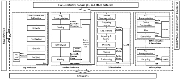
Figure 1. The system boundary of this study.
Download figure:
Standard image High-resolution image2.1. Forest management and log production
This stage includes forest growth, three major forest operations (i.e. site preparation and planting, fertilization, and logging), and the decay of harvest residues, which comprise the major sources of carbon sequestration and GHG emissions. The forest growth sequesters the carbon from the atmosphere, while the GHG emissions come from forest operations and the decay of harvest residues [42]. The life-cycle GHG emissions from forest operations were estimated based on the usage of fuels and chemicals (e.g. fertilizers, herbicides) of each operation and their upstream burdens (see table 1 and SM section 2.1). Key parameters with variations and uncertainties are shown in table 2 (details for distribution tests in SM section 2.3). In this study, the harvest residues (mainly referring to limbs and tops) decay on the forest land and slowly release GHG emissions which were modeled by an exponential decay model (SM section 2.4) [43, 44].
Table 1. Diesel consumption and chemical usage of forest operations.
| Unit | Value | |
|---|---|---|
| Diesel consumption in fertilization and herbicide application [45] | kg ha−1 a | 7.5 |
| Diesel consumption in planting [45] | kg ha−1 | 23.4 |
| Nitrogen fertilizer usage [46] | kg N ha−1 | 103.1 |
| Phosphorus fertilizer usage [46] | kg P2O5 ha−1 | 12.8 |
| Herbicide usage (glyphosate) [45] | kg ha−1 | 1.36 |
Table 2. Key parameter values and assumed distributions in log production based on literature data.
| Unit | Mean value | Minimum | Maximum | Assumed distribution | |
|---|---|---|---|---|---|
| Live tree moisture content [47, 48] | % dry | 88.5 | 75 | 102 | Uniform [75 102] |
| Stem wet density [49–51] | kg m−3 | 881 | 833 | 929 | Uniform [833 929] |
| Diesel consumption of site preparation [45, 52–54] | kg ha−1 a | 72.11 | 43.65 | 94.59 | Uniform [43.65,94.59] |
| Diesel consumption of logging [45, 52, 53, 55–65] | kg m−3 log | 1.66 | 0.37 | 3.57 | Normal N(1.40, 0.62) |
| Carbon content of aboveground pine tree [66–77] | % dry | 49.2 | 45.5 | 52.0 | Normal N(49.2, 2.12) |
The emissions from residue decay and logging, and carbon sequestration largely depend on the growth rate of the trees. In this study, the FASTLOB model [78] was used to simulate the stand-level loblolly pine (Pinus taeda L.) growth and yield. Two growth cases (GCs) were modeled with different site indices describing the forest site productivity as shown in table 3 [79]. The model generated annual aboveground biomass data (SM section 2.2) for one rotation (25 years). After 25 years, the trees were harvested with a clear cut (all standings are felled), generating saw logs as the main products and harvest residues. The logs under bark were transported to mills, which is a common industrial practice [80, 81]. This work does not consider alternative wood products such as pulpwood, lumber, and pellets, given the focus of this study on CLT. Those market-driving options for landowners largely depend on the forest economic and market conditions, which is beyond the scope of the study but could be explored and compared in future consequential LCA leveraging the results and data from this work.
Table 3. Assumptions of two growth cases based on representative forest practice [82, 83].
| Growth Case | Site index | Planting density (trees per ha) | Time of applying fertilizer | Rotation length | Thinning |
|---|---|---|---|---|---|
| GC1 | 60 | 1680 | Year 10 &16 | 25 | None |
| GC2 | 90 | 1680 | Year 10 &16 | 25 | None |
The results of the FASTLOB model are shown in figure 2 for 1-ha accumulative aboveground biomass in two GCs by logs and harvest residues. GC2 has higher log output (443 metric tonnes) and more harvest residues (111 metric tonnes) because of higher site productivity. After each rotation, logs are transported to lumber mills and residues are left on the ground. Note that this work is a stand-level analysis, and the fluctuations of forest carbon stock over 100 years at a landscape level are not considered. However, the results presented by this study can provide useful information for future landscape-level analysis that considers forest carbon stock changes.
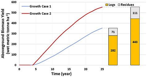
Figure 2. The growth and yield of 1-ha forest land per rotation for growth case 1 and 2.
Download figure:
Standard image High-resolution image2.2. Lumber production
After log production, logs with bark are transported to lumber mills with an assumed transportation distance, 92 km [84]. The main unit operations in lumber mills include sawing, kiln drying, planing, and energy generation for the dry kiln [81, 84]. The process parameters with variations are shown in table 4. The GHG emissions and primary energy consumption were estimated based on the upstream burdens and the emission factors of energy and fuels (see tables S1 and S5).
Table 4. Key parameters with variations in lumber production.
| Unit | Mean value | Minimum | Maximum | Assumed distribution | |
|---|---|---|---|---|---|
| Diesel consumption of hauling materials [49–51] | kg m−3 dried lumber | 3.6 | 1.7 | 5.5 | Uniform [1.7,5.5] |
| Gasoline consumption of hauling materials [49–51] | kg m−3 dried lumber | 0.23 | 0.03 | 0.23 | Uniform [0.03,0.43] |
| Bark mass fraction [85] | % | 10.5 | 9 | 13 | Uniform [9,13] |
| Lumber yield in sawing [84, 86–96] | % | 50 | 36 | 64 | Triangular 36, 50, 64 |
| Electricity consumption of sawing [84, 88, 97, 98] | kWh m−3 log input | 24.4 | 16.5 | 32.3 | Uniform [16.5,32.3] |
| Electricity consumption of kiln drying and kiln heat generation [84, 86, 88, 97, 99] | kWh m−3 lumber input | 26.9 | 17.9 | 35.8 | Uniform [17.9,35.8] |
| Lumber target moisture content [15, 19, 30, 86, 93, 100] | % (dry basis) | 12.5 | 6 | 19 | Triangular 6, 12.5, 19 |
| Overall energy efficiency for energy generation and drying [84, 88, 99] | % | 23.3 | 16.7 | 29.8 | Uniform [16.7,29.8] |
| Lumber drying shrinkage [101] | % | 9.14 | 4.37 | 15.96 | Triangular 4.37, 9.14, 15.96 |
| Electricity consumption of planing [84, 86, 88, 97] | kWh m−3 lumber input | 18.2 | 7.7 | 28.7 | Uniform [7.7,28.7] |
| Planing byproduct mass percentage [84, 86, 88, 102] | % | 17.8 | 13.8 | 21.8 | Uniform [13.8,21.8] |
2.2.1. Sawing.
Logs are first debarked, and the mass fraction of barks produced was assumed to be 9%–13% (see table 4). Then logs are sawn producing wet lumber and two byproducts (slabs/chips and wet sawdust). The lumber mass was determined by lumber yield in sawing (see table 4). The wet mass allocation of two byproducts was 82.1 wt% slabs/chips and 17.9 wt% wet sawdust [86]. In this study, all the slabs/chips were assumed to be sold to produce particle boards or other wood products [103, 104] that were excluded from the system boundary (see figure 1). Bark and wet sawdust, along with dry planner shavings and sawdust, were used for two alternative energy production cases (see below).
2.2.2. Kiln drying.
Wet lumber are sent to a kiln at 90 °C–120 °C (dry bulb temperature) to reach the targeted moisture content [99, 100]. Drying energy comes from either wood residues or natural gas. The fuel consumption for kiln drying was calculated as heat demand divided by the overall energy efficiency for energy generation and drying (see section 2.2.4 and SM section 3.1 for details). Table 4 also includes a parameter for lumber drying shrinkage due to moisture content reduction [101, 105].
2.2.3. Planing.
Planing processes wood to produce finished lumber in the required dimension and quality [97]. The process generates [106] dry sawdust and dry shavings/chips as byproducts/wastes [84, 97]. The dry sawdust was assumed to be 3.3 wt% of the total planing byproducts and the remainder were shavings/chips [97]. Then the dried lumber is stacked and ready to be transported to CLT producers.
2.2.4. Energy generation for kiln.
Either biomass fuels or a fossil fuel like natural gas can be combusted to generate energy for the dry kiln. In this study, a lumped parameter was used to cover the overall energy efficiency of kiln drying and energy generation, as shown in table 4.
Energy supply has direct impacts on the energy and GHG emissions of lumber production [97]. This study explored two energy supply scenarios. This energy recovery scenario combusted mill residues (bark, sawdust, and shavings/chips from planing) to supply energy needed by the dry kiln, which represents the situation where selling mill residues is not economically attractive (e.g. high transportation cost). Excessive residues were allocated to power generation. The sold-to-market scenario used natural gas to meet the energy demand of the dry kiln and sold mill residues to other manufacturers for DWP production (e.g. particle boards) [103, 104, 107]. The energy supplied by different fuels was estimated by the lower heating value (LHV) as documented in SM section 3.1. Note that mill residues have other choices (e.g. pellets, mulch) that highly depend on the economic drivers and should be analyzed on a case-by-case basis.
2.3. CLT production
In CLT production, lumber preparation is the first step. It includes lumber selection, grouping, re-cutting, and dust removal [30, 108]. The selected and grouped lumber is longitudinally end-jointed to make long continuous lumber [15]. In this study, the end-jointing type was assumed to be finger-jointing. Four-side planing is needed for the end-jointed lumbers to meet the thickness tolerance requirement for better bonding results [6, 15]. The lumber layered and glued is applied for face bonding [24]. Melamine formaldehyde (MF), a common resin, was assumed to be used in finger-jointing and face-bonding, and the MF quantity was collected from literature and shown in table 5 [15, 19, 29, 30]. To remove any excess resin and final uneven surfaces, planing or trimming is needed after pressing. As CLT panels are highly prefabricated products for fast erection and minimal onsite finishing, Computerized numerical control (CNC) is commonly used to cut CLT according to customized design [109]. The power consumption of CLT production was collected from literature and shown in table 5. The diesel consumption of hauling and conveying materials between unit operations was assumed 0.85 kg m−3 final CLT produced [49–51]. All the wood wastes were sent to landfill and the emissions by landfill decay were discussed in section 2.6. Table 5 shows all process parameters with variations for the CLT production.
Table 5. Key parameters with variations and uncertainties in the CLT production.
| Unit | Mean value | Minimum | Maximum | Assumed distribution | ||
|---|---|---|---|---|---|---|
| Lumber transportation from lumber mill to CLT producer [19, 30] | km | 265 | 91 | 438 | Uniform [91 438] | |
| Resin (MF) for finger-jointing and pressing [15, 19, 29, 30] | kg m−3 lumber input | 6.1 | 5.3 | 6.9 | Uniform [5.3,6.9] | |
| Planing shavings percentage [19, 30] | % m−3 CLT input | 4.0 | 3.6 | 4.5 | Uniform [3.6,4.5] | |
| End cutting waste percentage [19, 30] | % m−3 CLT input | 12.8 | 12.2 | 13.4 | Uniform [12.2,13.4] | |
| Total electricity consumption of CLT production [19, 29, 30] | kWh m−3 final CLT produced | 113.8 | 98.9 | 128.7 | Uniform [98.9128.7] | |
2.4. CLT construction and demolition
The transportation distances between CLT producers and construction sites were assumed to be 104–320 km [30]. This study estimated GHG emissions and energy consumption of construction and demolition based on the literature (see SM section 4) [23]. The building life span in this study was assumed to be 60 years [2, 23, 25, 110–112], and the carbon stored in buildings were included. This work does not include the energy consumption and GHG emissions of buildings' use phase, because they are driven by man factors such as architecture design and energy end-uses (e.g. heating and cooling facilities and electronic appliances) [113, 114] that are not necessarily related to the construction materials. Such environmental burdens need to be addressed on a case-by-case basis given large variations across different building types and designs, user behaviors, energy management strategies, and allocation methods [2, 27].
2.5. CLT recycling
Previous studies indicated that CLT can be partially recycled but the real-world practice is still limited [4, 23, 25]. Due to the lack of data, this study developed two conceptual cases to explore the impacts of recycling (assumed 50% recycling rate) compared with landfilling (0% recycling rate) [4, 23, 25, 115]. The landfilled CLT panels come from either the building site (as demolition waste) or a CLT recycling plant (as waste from recycling). The transportation distances were assumed to be the same as that from CLT producer to construction sites. GHG emissions and energy consumption of the CLT recycling plant were assumed to be 50% of the normal producing process as recycling does not need end-jointing, layering and gluing, or pressing.
2.6. Wood waste landfill
Landfilled wood wastes emit GHG through decay over a very long period, affecting the overall carbon analysis [116]. Unlike the decay on forest land, landfill decay emits a large amount of CH4 that has a much higher global warming potential (GWP) characterization factor than CO2 (100-year GWP for CH4 is 28) [117, 118]. In this study, the GHG emissions from landfill decay were estimated based on the Intergovernmental Panel on Climate Change (IPCC) First Order Decay (FOD) method (see SM section 5) [116].
2.7. Scenario analysis
The scenarios, as shown in table 6, were designed to explore counterfactual alternatives related to forest growth, energy supply, and end-of-life options of CLT, three aspects that have large impacts on the carbon and energy flows of CLT systems. The impacts of variations in other process parameters were explored by Monte Carlo simulation [30]. For each scenario, Monte Carlo simulation was performed for 500 iterations using the probability density functions of parameters as shown in tables 2, 4 and 5.
Table 6. Scenario analysis.
| Forest Growth Cases in Log Production | Mill Residues Utilization Cases in Lumber Production | CLT Recycling | |||
|---|---|---|---|---|---|
| Case Number | Site Index | Mill Residues for Energy Recovery | Mill Residues Sold to Market | Recycling Rate | |
| Scenario 1 | GC1 | Low | X | 0% | |
| Scenario 2 | X | 50% | |||
| Scenario 3 | X | 0% | |||
| Scenario 4 | X | 50% | |||
| Scenario 5 | GC2 | High | X | 0% | |
| Scenario 6 | X | 50% | |||
| Scenario 7 | X | 0% | |||
| Scenario 8 | X | 50% | |||
3. Results and discussion
The results in figure 2 were used to simulate the dynamic carbon flows for 8 scenarios across 100 years for 1-ha forest land. Given the similar trends across all eight scenarios, figure 3 only shows the results of Scenario 6 (see SM figures S2–S9 for the other scenarios). Carbon flows related to CLT and byproducts are shown separately in figures 3(a) and (b) for better readability. In figure 3, positive values (solid lines) represent GHG emissions, while negative values (dashed lines) represent sequestrated CO2. The shaded area of each line indicates the result ranges (5th percentile (P5) to 95th percentile (P95)) caused by uncertainty. The line represents the mean value. The timeline starts with planting pine at year 0 for a 25-year rotation. The CO2 sequestrated by aboveground live trees (light blue dashed line in figure 3(a)) returns to zero after logging every 25 years. After harvest, logs are transported to the lumber mill, while forest residues are left on land (gray dashed line in figure 3(b)) that decays and generates GHG (solid gray line in figure 3(b)). Then logs are manufactured to be CLT panels, serving as a carbon storage pool (green dashed line) one year after the logging and correspondingly emit the GHG due to the CLT manufacturing process (solid green line) in figure 3(a). In year 86, 60 years after the manufacturing, the CLT manufactured from the first rotation is demolished and the carbon stored in that CLT consequentially decreases.

Figure 3. 100-year accumulative GHG flows of 1 ha pine forest land of scenario 6. (a) GHG emissions related to CLT panels; (b) GHG emissions related to byproducts and wood waste. CLT manufacturing shown in (a) includes GHG emissions from lumber production and CLT production.
Download figure:
Standard image High-resolution imageThe carbon stored in landfill waste is indicated by the black dashed line in figure 3(b). This carbon stock slowly releases GHG emissions by landfill decay (solid black line in figure 3(b)). The end-of-life can be complex given the variety of DWP and their fate (e.g. landfilled with or without energy recovery, or burned for energy generation), but these alternatives are outside the system boundary of this study, and should be analyzed on a case-by-case basis.
Figure 3 shows that from a 1-ha perspective, GHG emissions are dominated by CLT manufacturing and decay from landfill and harvest residues. GHG emissions from forest operations, CLT construction and demolition, and CLT recycling are minimal (see figure 3(a)). This trend is consistent across all scenarios.
The comparison of 8 scenarios (see figures S2–S9) has three conclusions. First, over 100 years, higher forest productivity leads to the higher volume of produced CLT and more carbon storage that increases both downstream emissions and sequestration. For example, the carbon stored in CLT panels in Scenario 6 (GC2, high forest productivity) is 56% higher than that in Scenario 2 (GC1, low forest productivity), but Scenario 6 has 57% higher GHG emissions from CLT manufacturing than that in Scenario 2 (all based on mean value of GHG). Second, GHG emission differences in CLT manufacturing are driven by the mill residue options. For example, the mean CLT manufacturing GHG emissions in Scenario 6 (energy recovery in figure 3(a)) is 36% higher than Scenario 8 (sold-to-market in figure S9) in year 100. The mill residue options also affect carbon sources in CLT manufacturing. In Scenario 6, ~14% of CLT manufacturing GHG emissions are fossil-based; in Scenario 8, over 99.5% of those are fossil-based.
Besides CLT manufacturing, the largest and relatively near-term GHG emissions are from forest residues decay (266 metric tonnes in figure 3(b)), while a delayed but significant source is from landfill decay (151 metric tonnes). These two sources account for 48% of the total 100-year GHG emissions and justify the carbon benefits of converting residues to bioenergy products (e.g. biofuel, pellets, biochar) [36, 76, 119–125].
Figure 4 shows the life-cycle GHG footprints (all fossil- and biogenic-based GHG emissions minus the total CO2 sequestrated from the atmosphere) for 1-ha land over 100 years. The site productivity or growth rate has the dominant impact, as shown by the significant differences between slower growing GC1 scenarios (Scenario 1–4) and faster growing GC2 scenarios (Scenario 5–8). This observation highlights the importance of improving forest productivity from a life-cycle GHG perspective for CLT systems.
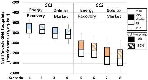
Figure 4. Net life-cycle GHG footprints of 1-ha forest land for 1 rotation in 100 years in varied growth cases (GC1 or GC2), mill residue end-of-life options (for energy recovery or sold to market), and CLT recycling rates (0% or 50%). Mill residues are sold to produce wood products (e.g. particle boards) by other manufacturers in the 'Sold to Market' scenario.
Download figure:
Standard image High-resolution imageAnother, and somewhat surprising, observation is the greater net GHG emissions for the scenarios using mill residues for energy recovery, compared to the scenarios selling residues to market. This phenomenon is caused by two factors. First, energy recovery immediately releases carbon that otherwise would be stored in DWP made from mill residues (e.g. 444 metric tonne CO2 in DWP in Scenario 6 (energy recovery) versus 769 metric tonnes in Scenario 8 (sold to market)). Second, energy recovery generates more GHG emissions given the lower LHV of mill residues than that of natural gas (see SM section 3.1). Hence, energy recovery case uses renewable energy (mill residues) and results in higher net GHG emissions, while sold-to-market case uses fossil fuel (natural gas) and sells mill residues to produce wood products, and results in lower net GHG emissions but higher fossil-based GHG emissions (see figure 5).

Figure 5. Fossil-based life-cycle GHG emissions of 1-ha forest land for 100 years in varied growth cases (GC1 or GC2), mill residue end-of-life options (for energy recovery or sold to market), and CLT recycling rates (0% or 50%). Mill residues are sold to produce wood products (e.g. particle boards) by other manufacturers in the 'Sold to Market' scenario.
Download figure:
Standard image High-resolution imageFinally, figure 4 shows the effects of the 'end-of-life' scenarios (50% recycled/50% landfilled versus 100% landfilled). The recycling rate does not show a significant impact on the net GHG emissions, which can be explained by the relatively modest amount of CLT that reached the end of life within the 100-year timeframe, and the relatively slow decay in the landfill. See SM section 7 for primary energy results.
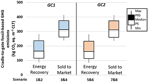
Previous LCA studies used cradle-to-gate system boundary on 1 m3 CLT basis [19, 29, 30], thus the results of this study were converted to the same system boundary and functional unit for a consistent comparison, as shown in figure 6 Several observations can be derived. First, the effects of different GCs are minimal on 1 m3 basis (less than 2%) because forest growth only affects log production. Second, energy recovery reduces fossil-based GHG emissions by 47%–48%, due to the reduced use of natural gas (see SM figure S13 for primary energy results). The results of previous studies using a cradle-to-gate system boundary are 80.0–206.3 kg CO2 eq. m−3 CLT [19, 29, 30]. They use carbon neutral assumption and thus only include fossil-based emissions (details of literature data are available in SM section 1). Variations in the results of previous studies are mainly due to differences in manufacturing processes, energy supply, forest characteristics, and transportation. Our results for the fossil-based GHG emissions (113.1–375.4 by P5-P95 across all cases) are consistent with the previous studies.
Figure 6. Cradle-to-gate (CLT producer gate) fossil-based GHG emissions of 1 m3 CLT produced.
Download figure:
Standard image High-resolution image
This work presents dynamic carbon flows of the integrated forest and CLT systems, which are critical knowledge to identify effective strategies for maximizing the system-wide carbon benefits of using the forest for CLT production. Those strategies range from process design and optimization for CLT manufacturing to forest and waste management. Although this work does not include the use phase of buildings, the presented results and data provide a foundation for future LCAs or environmental analysis of CLT buildings. The upstream and downstream burdens of CLT products estimated in this study allow future LCA practitioners or architects to explore CLT coming from different forests, manufacturers, and being treated in different end-of-life scenarios. This is also the first work that highlights the significance of emissions from forest residues decay and wood waste landfills, indicating the importance of including those emissions and life-cycle stages in the future LCAs for different wood products.
4. Conclusions
This study developed a dynamic cradle-to-grave modeling framework and examined the carbon and energy flows of the CLT life cycle over 100 years. Varied forest GCs, CLT manufacturing variables, and CLT recycling cases were investigated to explore their effects on the carbon and energy flows per 1-ha forest land basis and 1 m3 basis. On a 1-ha basis, higher forest productivity leads to significantly lower net life-cycle GHG emissions over 100 years. The largest GHG emission source is CLT manufacturing, including lumber production and CLT production. The heat source for lumber drying has large impacts on GHG emissions. Converting lumber mill residues to DWP reduces the overall 1-ha GHG emissions compared to burning the residues for drying lumber but largely increases the fossil-based GHG emissions. The decay of wood wastes (either from forest residues or a landfill) generates significant GHG emissions over 100 years, highlighting the importance of utilizing wood wastes in a more valuable and efficient way. Increasing the CLT recycling rate from 0% to 50% slightly reduces the 1-ha life-cycle GHG emissions. This small reduction is due to only one recycling activity taking place during the 100-year period.
This study conducts extended research on the cradle-to-gate GHG emissions and energy consumption of 1 m3 CLT produced for a comparison with the literature. On a 1 m3 CLT basis, different GCs have minor impacts on the results, which contrasts to the conclusion on a 1-ha basis. Because the two forest growth cases only affect the results of log production, but not other life cycle stages. The fossil-based GHG emissions are largely affected by the options of mill residues. Specifically, 113.1–236.3 kg CO2 eq. m−3 (P5–P95) of fossil-based GHG emissions were generated when using mill residues for energy recovery and 260.3–375.4 kg CO2 eq. m−3 (P5–P95) were generated when selling mill residues to produce wood products.
Acknowledgments
This work is in part supported by the award 70NANB18H277 from the National Institute of Standards and Technology, U.S. Department of Commerce. The statements, findings, conclusions, and recommendations are those of the author(s) and do not necessarily reflect the views of the National Institute of Standards and Technology or the U.S. Department of Commerce. We thank Dr. Joshua D. Kneifel from NIST for providing the feedback for the manuscript. This work is funded in part by a joint venture agreement between the USDA Forest Service, Forest Products Laboratory, and the U.S. Endowment for Forestry & Communities, Inc., Endowment Green Building Partnership—Phase 1, no. 16-JV-11111137-094.
Data availability statement
All data that support the findings of this study are included within the article (and any supplementary information files).