
Abstract
A beam delivery system using a single-radius-beam-wobbling method has been used to form a conformal irradiation field for proton radiotherapy in Japan. A proton beam broadened by the beam-wobbling system provides a non-Gaussian distribution of projection angle different in two mutually orthogonal planes with a common beam central axis, at a certain position. However, the conventional initial beam model for dose calculations has been using an approximation of symmetric Gaussian angular distribution with the same variance in both planes (called here a Gaussian model with symmetric variance (GMSV)), instead of the accurate one. We have developed a more accurate initial beam model defined as a non-Gaussian model with asymmetric variance (NonGMAV), and applied it to dose calculations using the simplified Monte Carlo (SMC) method. The initial beam model takes into account the different distances of two beam-wobbling magnets from the iso-center and also the different amplitudes of kick angle given by each magnet. We have confirmed that the calculation using the SMC with NonGMAV reproduced the measured dose distribution formed in air by a mono-energetic proton beam passing through a square aperture collimator better than with the GMSV and with a Gaussian model with asymmetric variance (GMAV) in which different variances of angular distributions are used in the two mutually orthogonal planes. Measured dose distributions in a homogeneous phantom formed by a modulated proton beam passing through a range shifter and an L-shaped range compensator, were consistent with calculations using the SMC with GMAV and NonGMAV, but in disagreement with calculations using the SMC with GMSV. Measured lateral penumbrae in a lateral direction were reproduced better by calculations using the SMC with NonGMAV than by those with GMAV, when an aperture collimator with a smaller opening was used. We found that such a difference can be attributed to the non-Gaussian angular distribution of the initial beam at a lateral position for the beam-wobbling system. Calculations using the SMC with NonGMAV are effective to reproduce dose distributions formed by a beam-wobbling system more accurately than that with GMSV or that with GMAV.
Export citation and abstract BibTeX RIS
General scientific summary For proton radiotherapy, a proton beam broadened by a beam-wobbling delivery system provides non-Gaussian distributions of projection angle different in the two orthogonal projected planes. However, the conventional initial beam model for dose calculations has been using an approximation of a Gaussian angular distribution with symmetric variance (GMSV) in both planes. Therefore we have developed a more accurate model defined as a non-Gaussian model with asymmetric variance (NonGMAV), and applied it to dose calculations using the simplified Monte Carlo (SMC) method. We verified the calculation accuracy by comparing measured dose distributions in air, and in a homogeneous phantom. We confirmed that the SMC with the NonGMAV reproduced the measured dose distributions clearly better than the SMC with the GMSV. In conclusion, the SMC with the NonGMAV will be an effective tool for accurate dose calculations for a proton beam-wobbling delivery system.
1. Introduction
The purpose of radiotherapy is to eradicate a malignant tumor by giving a lethal dose to it while sparing normal tissues surrounding the tumor by minimizing dose to them. The proton beam is an effective tool for that purpose due to the better dose localization by the characteristic depth–dose distribution with a Bragg peak.
A beam delivery system is required to conform a dose distribution to a target volume while reducing doses to the surrounding normal tissues. Broad beam delivery systems spread the proton beam laterally by one of a number of methods and longitudinally by a ridge filter or a rotating wheel to cover the target volume. In addition, proton ranges are adjusted uniformly by a range shifter and position-to-position by a range compensating bolus to conform the distal boundary of dose distribution to that of the target volume. A patient aperture collimator defines the lateral extent of the dose distribution.
One type of the lateral beam-spreading methods is a double scattering method, where a uniform first scatterer is followed by a non-uniform second scattering system to form a uniform lateral dose distribution in the target volume (Koehler et al 1977, Gottschalk et al 1991, 2008, Takada 1994, 2002). The other is a circular beam-wobbling method (Renner and Chu 1986, Chu et al 1993, Kanai et al 1999) or a uniform raster scanning method (Zheng et al 2011). In Japan, a beam-wobbling system consists of a pair of beam-wobbling magnets drawing a single circle of beam-center orbit and a uniform scatterer (we will call it a single-radius-beam-wobbling system hereafter). An example of the system installed in a proton rotating gantry system of the National Cancer Center Hospital East (NCCHE) is shown in figure 1. Here, we define a Cartesian coordinate system fixed to the rotating gantry so that the central beam direction is the z-direction, a lateral direction parallel to the rotation axis is the y-direction and a direction perpendicular to both y- and z-directions is the x-direction.
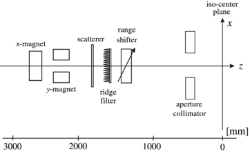
Figure 1. Schematic layout of the beam-wobbling delivery system at NCCHE.
Download figure:
Standard image High-resolution imageFor each beam delivery system, an accurate and fast dose calculation model is required for proton treatment planning. Each dose calculation model uses an initial beam model in which the angular distribution of protons is given for each lateral position on the starting plane of calculation. To save calculation time, the scattering effect of the beam line devices on the beam phase space is reduced to an effective proton source. The effective source model was developed and applied successfully to the double scattering system (Hong et al 1996, Szymanowski et al 2001, Kohno et al 2002, 2003, Hotta et al 2010). The effective proton source is characterized by two parameters: a distance between the iso-center and the effective source position, and the lateral size of the effective source, which can be calculated by the Fermi–Eyges theory (Eyges 1948) or be determined by measurements (Hong et al 1996, Szymanowski et al 2001). Since scattering occurs symmetrically around the incident beam direction, the two effective source parameters in the two mutually orthogonal lateral directions are the same.
On the other hand, in the single-radius-beam-wobbling system, the beam is kicked in the x-direction by one of beam-wobbling magnets and then kicked in the y-direction by the other so that the beam center draws a circle with a beam-wobbling radius around the iso-center. Then the beam is scattered by a uniform scatterer to form a lateral fluence distribution of Gaussian shape with an rms σ. If the beam-wobbling radius and the σ are properly selected, a uniform dose distribution is formed in the central region. Since the kick angles in the beam-wobbling magnets are determined by the azimuthal angle position of the beam center on the circle and generally different in x–z and y–z planes, the angular distribution of protons at a certain position is different from that for the double scattering system and cannot be approximated well by the Gaussian distribution. In addition, different kick positions and amplitudes of kick angle given in the beam-wobbling magnets produce different angular distributions in x–z and y–z planes at a lateral position on the starting plane. Thus a more accurate initial beam model other than the effective source model is required to calculate dose distributions more accurately for the beam-wobbling system.
Tomura et al (1998) developed an initial beam model for the single-radius-beam-wobbling system and applied it to carbon cancer therapy at the Heavy Ion Medical Accelerator in Chiba (HIMAC). They obtained a formula for the angular distribution at a position (x, y). The formula has two parameters: a beam-wobbling radius and a distance between the kick position in the beam-wobbling magnet and the point of interest or an amplitude of kick angle, equivalently. Whereas they assumed that the beam is kicked in x- and y-directions at the same point in a single beam-wobbling magnet for simplicity, the beam, in fact, is kicked in the x-direction at the middle position of the one magnet and is then kicked in the y-direction at that of the other magnet. Such an approximation of the single kick in a virtual beam-wobbling magnet placed at the middle position between the actual two magnets seems to be relatively reasonable to reproduce the dose distribution in the lateral penumbra region for about a 10 m long HIMAC carbon beam line, since the distance between the beam-wobbling magnets is relatively short compared with the average distance of the beam-wobbling magnets from the iso-center. Yet such an approximation may produce a noticeable effect on the dose distribution for a typical proton beam line with about a one-third length of the carbon beam line. Actually, we found the difference of dose distribution in the lateral penumbra region between x- and y-directions for the proton gantry beam line at the NCCHE. In addition, although Tomura et al obtained an accurate angular distribution, they only calculated the average and variance of the angular distribution for each lateral position (x, y) and approximated the angular distribution by a Gaussian distribution with the average and variance. In fact, the angular distribution is much different from the Gaussian distribution. Therefore such an approximation may affect the accuracy of dose calculations.
Kanematsu et al (1998, 2006) applied the initial beam model to proton dose calculations using the pencil beam algorithm (PBA) for a beam-wobbling system. The PBA calculates a dose distribution by superposing dose deposits of individual pencil beams. They used the Gaussian distribution function as the angular distribution of the incident beam at the (x, y) position. They took into account the actual geometry of the beam-wobbling magnets to calculate the average projection angles of incident proton beam in x–z and y–z planes. However, the variances of projection angles of incident proton beam were taken as the same value both in x–z and y–z planes. Use of the Gaussian approximation and of the same variance may affect the accuracy on the dose calculations especially for the shorter proton beam line.
Therefore we have developed an accurate initial beam model for the proton beam-wobbling system. In the model, we take into account the actual geometry of beam-wobbling magnets and use an accurate angular distribution function instead of the Gaussian approximation. Then we measured proton dose distributions in a number of different conditions and compared the results with the accurate model and two other approximate Gaussian models to verify those accuracies.
2. Materials and methods
2.1. Initial beam models
2.1.1. Non-Gaussian model with asymmetric variance (NonGMAV)
A concise derivation of the proton angular distribution at a lateral position (x, y) is given for the beam-wobbling system as follows. Details can be consulted in Tomura et al (1998). Notice that the beam-center orbit in a plane perpendicular to the central axis of beam line is generally an ellipse instead of a circle described in the reference, since we take into account the actual geometry of a pair of beam-wobbling magnets.
When we power off beam-wobbling magnets, the angular distribution function fwob, off(x, y, θx, θy) of protons at a lateral position (x, y) for a certain longitudinal position along the beam axis can be described by the Fermi–Eyges theory (Eyges 1948) as
where θx, θy are projection angles in x–z plane and y–z plane, respectively. The σ11 is the projected spatial variance, σ12 is the projected spatial-angular covariance and σ22 is the projected angular variance.
While a magnetic field in one of the beam-wobbling magnets orients in y-direction to bend the beam in the x–z plane and varies with time as cos ωt, in the other beam-wobbling magnets it orients in the x-direction to bend the beam in the y–z plane and varies with time as sin ωt. We define a phase ϕ as ωt , where ω is the angular frequency of beam wobbling. When we power on the beam-wobbling magnets, the angular distribution function fwob, on (x, y, θx, θy) at a lateral position (x, y) can be expressed by integrating the fwob, off along the wobbling trajectory as
where the Rw, x and Rw, y are axis lengths in the x- and y-directions of the ellipse that the beam center draws by being kicked by the beam-wobbling magnets, respectively. Lw, x and Lw, y are distances between the longitudinal starting point of calculation and the center of each beam-wobbling magnet giving a kick in the x- or y-directions, respectively. In our initial beam model, the accurate formula (2) is used for generation of the projection angles for the individual initial protons. We named the initial beam model as a NonGMAV.
2.1.2. Conventional initial beam model: Gaussian model with symmetric variance (GMSV)
The PBA has been applied to the proton dose calculation for beam-wobbling systems (Kanematsu et al 2006). The PBA needs a Gaussian angular distribution at each lateral position (x, y) on the starting plane of calculation. We define here the Gaussian initial beam model as a GMSV, which has been used so far.
In the GMSV, they used the fluence distribution and the Gaussian projected angular distribution with the different averages and the same variance in the x–z and y–z planes as given in Kanematsu et al (2006). The fluence distribution FGMSV(r) and the Gaussian projected angular distribution G(θx,θy; x, y) with the variance  can be expressed as,


where In(z) is an nth order modified Bessel function (n = 0, 1, 2). Although they took into account the actual geometry of the beam-wobbling magnets for the calculation, they approximated the central projection angles in the x–z and y–z planes of the Gaussian distribution by simple geometrical angles (x/Lw, x, y/Lw, y) instead of more accurate ones (Tomura et al 1998). In addition, they did not take into account the actual geometry of the beam-wobbling magnets but used an average distance Lw of the Lw, x and Lw, y, and a common beam-wobbling radius Rw to calculate the same angular variance in the x- and y-directions. Further, they also used the same approximation to calculate the fluence distribution as given by the equation (3).
2.1.3. Gaussian model with asymmetric variance (GMAV)
Although the same value is used as variances of the angular distribution in the x–z and y–z planes in the GMSV approximation, we can easily extend the GMSV to an initial beam model with different angular variances in the x–z and y–z planes. We obtain the angular variance in the x–z plane by substituting Lw, x and Rw, x for Lw and Rw, respectively, in formula (5). We also obtain the angular variance in the y–z plane by substituting Lw, y and Rw, y for Lw and Rw, respectively, in formula (5). We define the initial beam model using the different angular variances as a GMAV. In the GMAV, we need to modify the fluence distribution to take into account the elliptical orbit of the beam center. The modified fluence distribution used for calculations with GMAV, FGMAV(x, y), is represented as follow:

Note that the GMSV and GMAV neither represent the feature of non-Gaussian angular distribution nor take into account the actual geometry of beam-wobbling magnets accurately.
2.2. Simplified Monte Carlo method
We calculated dose distributions by using the simplified Monte Carlo (SMC) method with three types of initial beam model to verify the calculation accuracy.
The SMC method (Sakae et al 2000, Kohno et al 2002, 2003, Hotta et al 2010) calculates a dose distribution by tracking individual protons. The initial beam is characterized by a distribution function in an initial phase space. The SMC starts tracking a proton at the entrance of the range compensator (RC). For calculations, we assumed a proton beam line using the beam-wobbling method at NCCHE as shown in figure 1. The RC is made from polyethylene and placed on an aperture collimator. For calculation of range loss and scattering of individual protons in material, the RC and the brass aperture collimator of 60 mm in thickness are divided into segments with a thickness of 1 mm and 0.5 mm along the beam axis, respectively. The energy loss of a proton in a segment is calculated by using the water equivalent model (Chen et al 1979). The SMC uses a measured depth–dose distribution in water along the central axis of beam line to calculate dose deposition in the material. The trajectory of each particle undergoing multiple Coulomb scattering in materials is tracked. Scattering projection angles are given by random numbers according to a normal distribution with a standard deviation calculated by the Highland formula (Highland 1975, 1979, Gottschalk et al 1993). We use actual radiation lengths depending on materials for calculation of scattering angles. The number of protons generated on the starting plane of calculation is determined so that the statistical error in the central region is within 0.5% rms of the central dose.
We have two reasons why we use the SMC method for the verification. First, we needed to use a dose calculation model based on a Monte Carlo method since the phase space of initial beam model using the NonGMAV have a distribution form other than the Gaussian form. Second, we intend to replace the conventional PBA used in the current treatment planning system at NCCHE by the SMC method that can improve the dose calculation accuracy within a practical time. For the double scattering system, which is adopted in another gantry beam line at NCCHE, the SMC has already been implemented in the treatment planning system for clinical use (Hotta et al 2010). In addition, the SMC has been verified to calculate a dose distribution for clinical case within a practical time by use of graphical processing units (Kohno et al 2011). With the successful results, we also intend to implement the SMC in the treatment planning system for the beam-wobbling method. Since the SMC can use an initial beam model with general stochastic distributions like NonGMAV, we expect that the SMC with the NonGMAV will be a beneficial tool for dose calculation for the beam-wobbling system.
2.3. Experiment apparatus
We verified calculation accuracy of the SMC with various initial beam models by comparing calculation results with measurements of proton dose distribution for the beam-wobbling delivery system at NCCHE as shown in figure 1. We used a 235 MeV proton beam extracted from the cyclotron at the NCCHE for all measurements.
A PTW 2D Array seven29™ was used for measurements of dose distribution (Spezi et al 2005, Hotta et al 2010). It is a two-dimensional detector matrix containing 729 vented ionization chambers in 10 mm pitch 27×27 array developed by ®PTW Freiburg GmbH. The sensitive volume of a unit chamber is 5 mm × 5 mm × 5 mm. The reference point is located 0.5 mm from the entrance surface of the detector and the offset thickness from the entrance surface to the center of the sensitive volume is 8 mm in water equivalent length. We repeated dose measurements three times in a single condition and used the averaged value as the dose at each point to reduce the uncertainty of dose measurement. Note that we are only interested in relative dose distribution in this study and the uncertainty of measured relative dose in the central region is estimated to be 0.35% rms of the central dose.
To compare the calculation results with measurements under the same conditions, we corrected the calculation depths by the offset thickness when calculating the dose distributions. We also convolved the calculation results with the detector cell size of 5 mm × 5 mm.
2.4. Measurement of lateral dose distributions under an open beam condition
We measured a lateral dose distribution formed by 235 MeV protons passing through an aperture collimator, at the iso-center in air. The distance between the bottom face of the aperture collimator and the iso-center was 250 mm. We used one of the three aperture collimators with a square opening of different sizes: 175×175, 100×100 and 50×50 mm2 for each measurement. Neither a ridge filter nor a range shifter was used for the measurements. Since the chamber pitch was 10 mm, we shifted the detector by 2.5 mm in the x- or y-directions, one at a time, by moving the patient couch to obtain a dose distribution with a sampling pitch of 2.5 mm.
We obtained the 80–20% lateral penumbra width of the measured dose distributions by using a polygonal line connecting the measured points in the penumbra region. The measured lateral penumbra width was compared with the calculated one to verify the calculation accuracy.
2.5. Measurement of dose distributions in a homogeneous slab phantom formed by a proton beam passing through a L-shaped range compensator
For evaluating accuracy of the SMC with the three initial beam models, we measured lateral dose distributions formed by a 235 MeV modulated beam passing through both a range shifter and a L-shaped RC, at various depths in a homogeneous phantom made from polyethylene. We formed the spread-out Bragg peak (SOBP) of 60 mm in width by passing a mono-energetic 235 MeV proton beam through a ridge filter made from aluminum alloy. Then the beam was range-shifted by a binary range shifter made from acrylic resin of 60 mm in thickness. The structure of the L-shaped RC and experimental layout are shown in figure 2. The L-shaped RC made from polyethylene was mounted on the aperture collimator with a square opening of 100×100 mm2. Measurements were made with a lateral sampling pitch of 5 mm.

Figure 2. An experimental arrangement is shown for measurements of dose distribution in the x-direction using a stack of slab phantoms, a L-shaped RC and an aperture collimator. We also measured dose distribution in the y-direction under the same arrangement by replacing the L-shaped RC with the structure in the x-direction by that in the y-direction.
Download figure:
Standard image High-resolution imageA stack of the phantom slabs was mounted on the detector to measure the dose distribution at each depth as shown in figure 2. Lateral dose distributions were measured at depths of z = 0, 35, 69, 98, 128 and 152 mm. When phantom stacks with different total thicknesses were mounted, we fixed the distance between the bottom surface of the aperture collimator and the entrance surface of the phantom by adjusting the vertical position of the patient couch.
We used two types of the L-shaped RC to investigate the difference of lateral dose distributions in the x- and y-directions. While the one type has an L-shaped structure in the x-direction, the other type has the same structure in the y-direction. We performed a series of experiments using one of them and another series of experiments using the other.
2.6. Estimation of errors and its propagation to estimated lateral penumbra width and the effect of detector resolution
Uncertainty of measured relative dose in the central region for an individual chamber of the detector is 0.35% rms of the central dose. The chamber-to-chamber variation of signals is estimated to be 0.6% rms of averaged signals of the adjacent chambers by comparing a dose detected by a chamber, with doses detected by the surrounding eight chambers in a uniform irradiation field. Estimated rms error of the 80–20% lateral penumbra due to both errors is 0.1 mm. The same amount of error is also estimated due to the statistical error of SMC calculations.
We obtained intermediate data with a sampling pitch of 2.5 mm using the detector with a pitch of 10 mm by moving the patient couch on which the detector is mounted. We estimated the effect of the position error of the patient couch on the measured 80–20% lateral penumbra in the following way. We used the same open beam condition described in section 2.4 with an aperture collimator with a square opening of 100×100 mm2. We repeated the same process of penumbra measurement three times and obtained three values of penumbra. The rms error of lateral penumbra due to the position error of the patient couch is then estimated to be 0.1 mm. Then the overall error of measured penumbra is estimated to be about 0.14 mm rms.
Since the measured lateral dose distributions were convolved with the detector size of 5 mm, the measured lateral penumbra width differs from the actual one. To estimate the difference, we simulated the lateral dose distribution in a fall-off region by a Gaussian penumbra function, F(x), using a Gaussian error function with a variance σ2, erf(x), as shown in the following formula (7):

where x0 indicates a horizontal x-coordinate corresponding to the edge position of the aperture collimator. Then we investigated the influence of finite detector resolution on lateral penumbra. For that purpose, we convolved the F(x) for various values of σ with the detector size of 5 mm and obtained the relationship between the original lateral penumbra and that convolved with the detector resolution. For example, the penumbrae of 4, 6, 8, 10 mm correspond to the convolved penumbrae of 4.5, 6.4, 8.4, 10.3 mm, respectively. The maximum difference between the penumbra and convolved one is 0.5 mm when the penumbra is 5.7 mm with the opening size of aperture collimator of 175×175 mm2 in the y-direction.
3. Results
3.1. Lateral dose distributions under an open beam condition
Figure 3 shows comparisons of lateral dose distributions in the x- and y-directions between the measurements and calculation results obtained by using the NonGMAV when the aperture collimator with a square opening of 100×100 mm2 is used. The dose distributions are normalized by the dose averaged around the central beam axis (defined as 100%) for the aperture collimator with a square opening of 175×175 mm2. As shown in figure 3, the relative dose in the central region was approximately 5% higher than 100%. It indicates that protons scattered on the surface of the aperture collimator (we call such scattered protons edge-scattered protons hereafter) contribute more to the central dose when the aperture size is smaller (Titt et al 2008). The SMC with NonGMAV reproduced the central dose increment well within 1∼2% since the SMC can track such individual edge-scattered protons. On the other hand, the SMC tends to overestimate the rise of shoulder for the dose contribution near the field edge region.
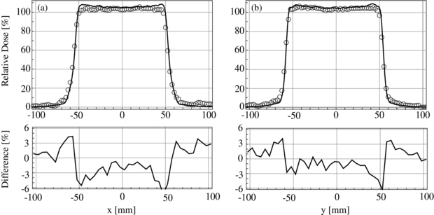
Figure 3. Lateral dose profiles of protons passing through an aperture collimator with a square opening of 100×100 mm2 in air. The open circles depict measurements and the solid lines depict calculation results obtained by using the SMC with the NonGMAV. Figures (a) and (b) show dose profiles in x- and y-directions, respectively. Since the measurement error is 0.35% rms of the central dose and smaller than the radius of circle, error bars are not displayed. The calculation error in the central region is 0.5% rms of the central dose. The lower part of each graph shows the errors obtained by subtracting calculations from measurements.
Download figure:
Standard image High-resolution imageWe also compare the 80–20% lateral dose penumbra widths between measurements and calculation results obtained by using the SMC with the three initial beam models for a number of aperture collimators with different opening sizes (figure 4). The measured lateral penumbra widths in the x-direction differ from those in the y-direction. The difference increases with reducing the opening size of the aperture collimator. The calculated lateral penumbrae using the GMSV are the same in both the x- and y-directions and cannot reproduce the measurements as shown in figure 4(a). On the other hand, the calculation results obtained by using the GMAV indicate the asymmetric lateral penumbrae and the results are clearly better than those obtained by using the GMSV as shown in figure 4(b). However, discrepancies remain, especially when an aperture collimator with the smallest opening size is used. In contrast, calculation results obtained by using the NonGMAV best reproduce all the measurement data compared with those from other initial beam models. Yet, there remains a penumbra difference of about 1∼1.5 mm between measurements and calculations even with the NonGMAV. Although edge-scattered protons on the aperture collimator may contribute to the difference, the discrepancy is open to further study.
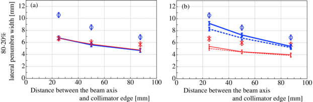
Figure 4. Comparisons of 80–20% lateral penumbra widths between measurements and calculation results for the different opening sizes of aperture collimator. The open circles and cross marks represent measurements in the x-direction and those in the y-direction, respectively. The blue thick and red thin lines depict calculation results in the x- and y-directions, respectively. The calculation results in (a) are obtained by using GMSV. The solid lines and dashed lines in (b) depict the calculation results obtained by using NonGMAV and GMAV, respectively. The error bar of measurements corresponds to three times the rms error, and the error bar of the calculation results corresponds to the statistical error.
Download figure:
Standard image High-resolution imageNote here that the calculation time with NonGMAV was 1.5∼2.1 times longer than those with the other two types of initial beam model due to the extra time for generation of the non-Gaussian angular distribution function.
3.2. Dose distribution in a homogeneous slab phantom formed by protons passing through a L-shaped range compensator
Figure 5 shows the comparisons of dose distributions in the x- and y-directions between measurements and calculation results obtained by using the NonGMAV. As shown in figures 5(a)–(c), calculations reproduce the measurements of the depth–dose profiles at (x, y) = (u, 0) and those at (x, y) = (0, u). The u is one of −25, 0, 25 mm. The distributions at (x, y) = (u, 0) are consistent with those at (x, y) = (0, u). On the other hand, the lateral dose distribution in the x-direction is different from that in the y-direction. When a polyethylene stack with a thickness of 35 or 98 mm is mounted on the detector, the measured dose distribution around the center in the x-direction is smoother than that in the y-direction (figures 5(d), (e) and (g), (h)). The difference can be attributed to the larger angular spread of incident protons in the x-direction than that in the y-direction. When a polyethylene stack with a thickness of 35 mm is mounted on the detector, the local dose increments due to edge-scattered protons are observed clearly in the edge region (figures 5(d) and (g)). The calculations reproduce the measurements well including the difference of dose distribution between the x- and y-directions and the local dose increments in the edge regions when a polyethylene stack with a thickness of 35 or 98 mm is used (figures 5(d), (e) and (g), (h)). In contrast, when we mount a polyethylene stack with a thickness of 152 mm on the detector, discrepancies are apparently observed in the flat region between the measurements and the calculation results (figures 5(f) and (i)). The apparent discrepancies can be attributed to the estimation error of the thickness of the polyethylene stack as follows. Since the lateral distributions are measured at the depth in the distal fall-off region of SOBP, the dose changes sensitively even with a small change of thickness of the polyethylene stack. Each polyethylene plate constituting the stack has an uncertainty of water equivalent thickness due to the uncertainty of material composition and thickness of the plate itself. We have confirmed that the apparent discrepancies could be improved in calculation by adjusting the thickness of polyethylene stack to within 1 mm.
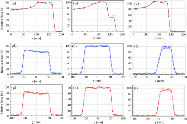
Figure 5. Comparisons of dose profiles in a homogeneous polyethylene slab phantom at different depths between measurements and calculation results obtained by using the SMC with the NonGMAV. The open circles and triangles represent measurements in x- and y-directions, respectively. The blue solid lines depict the SMC predictions in the x-direction and red dashed lines depict those in the y-direction. Figures (a)– (c) represent depth–dose profiles at x = 25 mm, 0 mm, −25 mm on y = 0 mm plane and at y = 25 mm, 0 mm, −25 mm on x = 0 mm plane. Figures (d)– (f) are lateral profiles in the x-direction and figures (g)– (i) are those in the y-direction. Figures (d), (g) are lateral profiles at z = 35 mm, figures (e), (h) are lateral profiles at z = 98 mm and figures (f), (i) are lateral profiles at z = 152 mm. Since the estimated measurement error from three measurements is 0.35% rms of the central dose and it is smaller than the size of each mark, error bars are not displayed.
Download figure:
Standard image High-resolution imageThe calculated lateral dose distributions obtained by using the NonGMAV are also compared with those obtained by using the GMSV and GMAV to investigate the influence of the initial beam model on dose distributions.
First, we focus on the influence of the angular distributions different in the x- and y-directions on dose distributions. Figure 6 shows comparisons of a calculated dose distribution in the x-direction with that in the y-direction at z = 98 mm for SMC calculations with the three initial beam models. The results of calculation with the GMSV in the x- and y-directions provide very similar distributions in the central region. The dose differences of lateral dose distribution between the x- and y-directions are within a statistical error of 0.7% rms value (figures 6(a) and (d)). In contrast, noticeable differences are found in the central region of the dose distributions in the x- and y-directions when the dose distributions are calculated by using the GMAV (figures 6(b) and (e)) and NonGMAV (figures 6(c) and (f)). These results indicate that angular distributions different in the x- and y-directions influence the shape of lateral dose distributions not only under the simple open beam condition described in section 3.1 but also under the more complex beam condition in which protons pass through a ridge filter, a range shifter and an RC and a phantom material. In addition, since the differences of lateral dose distribution in the x- and y-directions remain in the deep region of the homogeneous phantom, it is important to take into account the difference of angular distribution in the x- and y-directions for dose calculations for the beam-wobbling system. Note that since the GMSV takes into account the difference of average angles in x- and y-directions, the dose distribution calculated by using the GMSV may be possibly influenced by the different averaged angles in the x- and y-directions. However, the comparisons of dose distributions shown in figure 6 indicate that the influence of different averaged angles in x- and y-directions on dose distribution is less than the statistical error. Therefore we found that the different angular variances in x- and y-directions dominantly influence the dose distribution.
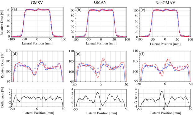
Figure 6. Comparison of lateral dose profiles at z = 98 mm between x- and y-directions. The open circles and triangles represent measurements in x- and y-directions, respectively. The solid and dashed lines depict the calculation results with the three initial beam models (left: GMSV, middle: GMAV, right: NonGMAV) in x- and y-directions, respectively. Figures (a)– (c) show overall lateral dose profiles and figures (d)– (f) show enlarged partial details of the central region. Each lower graph in figures (d)– (f) represents the subtraction of the calculated profiles in the y-direction from that in the x-direction. Since each calculated profile has a statistical error of 0.5% rms of the central dose, the subtraction has an error of 0.7% rms. The error bars are removed for ease of reading.
Download figure:
Standard image High-resolution imageNext, we focus on the influence of the non-Gaussian angular distribution on dose distributions. Figure 7 compares a calculated lateral dose distribution in the central region obtained by using the NonGMAV with that obtained by using the GMAV in each lateral direction. The difference between the dose distributions in both x- and y-directions falls within the statistical error. The fact indicates that the difference between the Gaussian and non-Gaussian angular distributions does not affect the dose distribution noticeably in this case. Consistency between calculated dose distributions with the GMAV and NonGMAV can be attributed to mitigation of the different effects of the initial beam conditions by the additional scatterings in other beam-modulating devices, especially the RC because the RC is located in the most downstream position of the beam line.
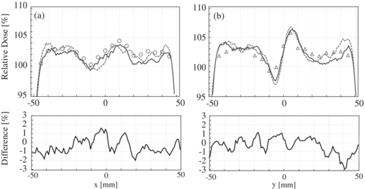
Figure 7. Lateral dose profiles in the central region in x- and y-directions at z = 98 mm. The open circles and triangles represent measurements in x- and y-directions, respectively. The solid lines depict calculated results obtained by using the SMC with the NonGMAV and dashed lines depict those with the GMAV. Figure (a) is a comparison in the x-direction and (b) is a comparison in the y-direction. Each lower graph in figures (a), (b) represents the subtraction of the calculated results with GMAV from that with NonGMAV. Since each calculation result has a statistical error with 0.5% rms of the central dose, the subtraction has an error with 0.7% rms. The error bars are removed for ease of reading.
Download figure:
Standard image High-resolution imageThe calculation time of the SMC with NonGMAV was approximately three times longer than that with other models. The calculation using a ridge filter is more time consuming than a mono-energetic condition because the initial beam model is calculated for protons passing through each different thickness of a ridge filter element.
4. Discussion
We found that measured lateral penumbrae in the x-direction are larger than those in the y-direction in air under an open beam condition. It means that an angular spread of protons in the x–z plane is larger than that in the y–z plane. The same indication was also observed in measured dose distributions of protons passing through an L-shaped RC, in a homogeneous slab phantom as shown in figure 5. In addition, we found that lateral penumbrae calculated by using the NonGMAV are larger than those calculated by using the GMAV as shown in figure 4, especially when the opening size of an aperture collimator is small. Further, the difference between the penumbra in the x-direction calculated by using the NonGMAV and that with the GMAV is larger than that in the y-direction for each of three opening sizes of aperture collimator. Any of these results can be attributed to the initial angular distributions of protons different in the x–z and y–z planes. Therefore it is important to produce the initial angular distribution of protons correctly as far as possible to reproduce the measured dose distributions using the calculation model.
Figure 8 shows calculated angular distributions of the two initial beam models, the NonGMAV and GMAV, at six lateral positions, (x, y) = (25, 0), (50, 0), (87.5, 0), (0, 25), (0, 50), (0, 87.5), on the bottom face of the aperture collimator, for the same geometry of measurements under the open beam condition described in section 2.4. The selected lateral positions correspond to the edge positions of the aperture collimators with different opening sizes used for the measurements. We noticed that each of the angular distributions calculated by using the NonGMAV has two peaks. The reason why we obtain such distributions follows in the next paragraph.

Figure 8. Calculated angular distributions at a lateral position (x, y) on the plane located upstream 250 mm from the iso-center. The solid lines depict the distributions calculated by using the NonGMAV. The dashed lines depict the distributions calculated by using the GMAV. Figures (a)– (c) show angular distributions in the x–z plane at (x, y) = (25, 0), (50, 0), (87.5, 0) mm. Figures (d)– (f) show angular distributions in the y–z plane at (x, y) = (0, 25), (0, 50), (0, 87.5) mm. These lateral positions correspond to edge positions of an aperture collimator used for measurements under an open beam condition.
Download figure:
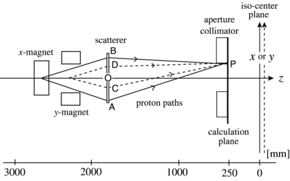
Standard image High-resolution imageProtons are kicked in the x-direction in one of the beam-wobbling magnets and then in the y-direction in the other so that the beam center draws an elliptical orbit on the scatterer plane perpendicular to the central axis of beam line. Figure 9 represents the proton paths projected on the x–z or y–z planes. Note that this figure merges two different setups in a single figure: the one setup has an aperture collimator with an opening in the x-direction (in the setup, the lateral axis is the x-axis), the other setup has an aperture collimator with an opening in the y-direction (in the setup, the lateral axis is the y-axis). In addition, the beam-wobbling magnets are displayed when the lateral axis is the x-axis. The axis length, 19.7 mm, of the ellipse in the y-direction, CO or DO, shown in figure 9 is shorter than that, 37.8 mm, in the x-direction, AO or BO, shown in figure 9. Those values result from the fact that the distance of 345.8 mm between the scatterer plane and kick point of the beam in the y-magnet is shorter than that of 768.0 mm between the scatterer plane and kick point of the beam in the x-magnet whereas the amplitude of kick angle of 56.8 mrad in the y-direction is larger than that of 49.2 mrad in the x-direction. In figure 9, a number of representative proton paths are shown incoming at P(x, y) on the bottom face of the aperture collimator: AP, BP in the x–z plane and CP, DP in the y–z plane. Each peak of projected angular distribution in the x–z plane on the positive side corresponds to the proton path AP approximately and that in the y–z plane corresponds to the proton path CP approximately. The other peak on the negative side in x-direction and that in y-direction correspond to the proton paths BP in the x–z plane and DP in the y–z plane approximately, respectively.
Figure 9. Projected paths of protons wobbled by x- and y-magnets in x–z or y–z planes.
Download figure:
Standard image High-resolution image
Using figure 9, we can explain (1) the difference of the angular widths between the x–z plane and y–z plane which is the cause of different penumbrae in the x- and y-directions, and (2) the peak-height dependence of the angular distribution on the edge position of the aperture collimator shown in figure 8, corresponding to the dependence of lateral penumbra on the opening size of the aperture collimator. Then we will discuss (3) the accuracy of approximation using the Gaussian angular distribution by using the figure 8.
Firstly, the larger width of angular distribution in the x–z plane than that in the y–z plane can be attributed to the longer axis length AB of the ellipse on the scatterer plane in the x-direction than that of CD in the y-direction, as shown in figure 9. The difference becomes apparent as the distance between beam-wobbling magnets and the iso-center becomes shorter. This is the reason why such effects can be seen in the proton beam line as short as about 3 m whereas they cannot be seen noticeably in the carbon beam line as long as about 10 m.
Secondly, we observe in the case of figure 8 that as the collimator edge moves away from the central axis of beam line to the positive side, (i) the position of two peaks shifts to the right-hand side and (ii) a height of the right-hand-side peak decreases and (iii) a height of the left-hand-side peak increases. The left-hand-side and right-hand-side peaks of angular distribution in the x–z plane approximately correspond to the proton path BP and that of AP, respectively. The angle between BP and the central axis of beam line gets smaller whereas the angle between AP and the central axis of beam line gets larger as the collimator edge moves away from the central axis of beam line to the positive side. Then the scattering probability of the left-hand-side peak increases corresponding to the scattering path BP and that of the right-hand-side peak decreases corresponding to the scattering path AP as the collimator edge moves away from the central axis of beam line to the positive side. This explains the facts (ii) and (iii) mentioned above. Then, the effective angular width of the initial beam gets smaller due to the decrease of the right-hand-side peak as the collimator edge moves away from the central axis of the beam line to the positive side. This fact can explain the trend of decreasing measured lateral penumbrae with the increasing opening size of aperture collimator.
Finally, since the separation between two peaks of the angular distribution in the y–z plane is smaller than that in the x–z plane, as shown in figure 8, due to the shorter axis length of the ellipse in the y-direction on the scatterer plane, the accuracy of Gaussian approximation in the y-direction is better than that in the x-direction. It indicates that a large discrepancy between the calculated angular distribution with the NonGMAV and that with the GMAV is observed when separation between the two peaks is large and the two peaks can be clearly identified. Then such a discrepancy can be seen most clearly when we use an aperture collimator with a small opening width. Actually, we found the two peaks most clearly in figure 8(a) corresponding to the aperture collimator with a square opening size 50×50 mm2 for measurement described in section 2.4. In fact, while calculations using the NonGMAV reproduced the measured lateral penumbrae in the x-direction very well, those using the GMAV cannot reproduce the measurements so well and the discrepancy was the largest when the opening size of aperture collimator was smallest.
Although we improved the calculation accuracy of lateral penumbra by using the NonGMAV, discrepancies of the penumbra remained between the calculation and measurement, as shown in figure 4. It is unclear at present whether the discrepancies are attributed to inaccuracy of the SMC or to that of modeling of the NonGMAV, or both. In the previous study (Hotta et al 2010), however, the accuracy of the SMC has been verified by comparing measured dose distributions in heterogeneous phantoms for a gantry beam line adopting the double scattering method at NCCHE. In the study, they found that the path rates of γ-analysis with 3%/3 mm tolerance was over 98% in most regions of the heterogeneous anthropomorphic phantom and they concluded that the accuracy of the SMC is sufficiently high for practical clinical application. In the present study, however, discrepancies of dose distribution partially remain between measurements and the SMC calculations. For example, the SMC slightly overestimates dose contributions in the field edge region as shown in figure 3. We will reveal the influence of the approximation in the SMC on dose distribution by comparison with calculations using a full Monte Carlo method like Geant and measurements in future study.
When we compared measurements with calculation results obtained by using the NonGMAV and the GMAV in a homogeneous slab phantom as shown in figures 6 and 7, the difference of calculation results with NonGMAV and GMAV is smaller than the statistical error. Considering comprehensively both the accuracy and calculation time between NonGMAV and GMAV, dose calculation with GMAV can be a reasonable tool in treatment planning especially when the PBA is used. However, the difference between lateral penumbra calculated by NonGMAV and that calculated by GMAV was largest in the x-direction when we used the collimator with the smallest opening size, as shown in figure 4. Then dose calculations with NonGMAV will serve to reduce calculation errors when an edge position of collimator in the x-direction is near the beam axis for clinical cases. For example, it corresponds to small field irradiation or irradiations of complex-shaped targets surrounding the central beam axis. In addition, we are interested in a situation when a collimator edge overhangs the beam central axis. We will investigate the dose differences between calculation with the NonGMAV and that with the GMAV in these clinical situations in future study.
5. Conclusion
We have developed an accurate initial beam model for the beam-wobbling delivery system and applied it to a dose calculation model using the SMC method. The model provides non-Gaussian angular distributions expressed in a projection angle with standard deviations different in x–z and y–z planes. Calculations using the SMC with the NonGMAV best reproduced measured dose distributions formed in air by a mono-energetic proton beam passing through a square aperture collimator. We also confirmed that the calculation results with the NonGMAV were in good agreement with measured dose distributions formed in a homogeneous slab phantom by a modulated proton beam passing through a range shifter and an L-shaped RC.
The observed differences between dose distributions in x- and y-directions cannot be reproduced well by calculations using the SMC with the conventional GMSV. Therefore we conclude that an accuracy of calculation with the GMSV is not enough to reproduce dose distributions delivered by the proton beam-wobbling system. In contrast, accuracy of the dose calculations was partially improved by using the GMAV. Thus for dose calculations using not only the SMC but also the PBA, we should at least use the GMAV as the initial beam model to improve the calculation accuracy. Transition of the GMSV to the GMAV is straightforward by only assigning different standard deviations for the projected angular distributions in the x–z and y–z planes.
In comparisons of lateral penumbra width in air between measurements and calculations, we observe that the accuracy of the calculations using the SMC with the GMAV deteriorates in the x-direction, as an opening size of aperture collimator becomes smaller. We found that the accuracy deterioration can be attributed to ignorance of the non-Gaussian angular distribution for the GMAV. In contrast, calculations using the SMC with the NonGMAV best reproduce the lateral penumbra widths for all the opening size conditions of the aperture collimator.
In conclusion, the SMC with the NonGMAV will be an effective tool for accurate dose calculations for a proton beam-wobbling delivery system.
Acknowledgments
We appreciate SHI Accelerator Service Ltd, for their support with the experiment. We are also grateful to members of Sumitomo Heavy Industries Ltd, for their advice to develop our calculation model.