
Abstract
Patient-specific image-based dosimetry is considered to be a useful tool to limit toxicity associated with peptide receptor radionuclide therapy (PRRT). To facilitate the establishment and reliability of absorbed-dose response relationships, it is essential to assess the accuracy of dosimetry in clinically realistic scenarios. To this end, we developed pharmacokinetic digital phantoms corresponding to patients treated with 177Lu-DOTATATE. Three individual voxel phantoms from the XCAT population were generated and assigned a dynamic activity distribution based on a compartment model for 177Lu-DOTATATE, designed specifically for this purpose. The compartment model was fitted to time-activity data from 10 patients, primarily acquired using quantitative scintillation camera imaging. S values for all phantom source-target combinations were calculated based on Monte-Carlo simulations. Combining the S values and time-activity curves, reference values of the absorbed dose to the phantom kidneys, liver, spleen, tumours and whole-body were calculated. The phantoms were used in a virtual dosimetry study, using Monte-Carlo simulated gamma-camera images and conventional methods for absorbed-dose calculations. The characteristics of the SPECT and WB planar images were found to well represent those of real patient images, capturing the difficulties present in image-based dosimetry. The phantoms are expected to be useful for further studies and optimisation of clinical dosimetry in 177Lu PRRT.
Export citation and abstract BibTeX RIS

Content from this work may be used under the terms of the Creative Commons Attribution 3.0 licence. Any further distribution of this work must maintain attribution to the author(s) and the title of the work, journal citation and DOI.
1. Introduction
Peptide receptor radionuclide therapy (PRRT) is an increasingly utilized treatment for patients with metastasized tumours of neuroendocrine origin (van Vliet et al 2013). The majority of these tumours express somatostatin receptors in abundance, enabling targeting with radiolabelled somatostatin analogues such as 111In-DTPA-Octreotide for diagnostic imaging (Krenning et al 1992, 1993) and 90Y- or 177Lu-labeled Octreotide/Octreotate for therapeutic purposes (Bodei et al 2004, Esser et al 2006, Kwekkeboom et al 2008). In PRRT, the organs at risk are the kidneys and bone marrow. One current recommendation to avoid long-term renal toxicity, based primarily on 90Y-Octreotide data, is that the cumulative biologically effective dose (BED) should not exceed 40 Gy for patients without pre-existing risk factors (Bodei et al 2008). The high inter-patient variability in uptake and retention of activity has motivated clinical research studies including patient-specific dosimetry, such as the Iluminet trial (EudraCT no. 2011-000240-16) in which our centre participates.
In general, patient-specific renal dosimetry in PRRT is based on image data obtained by scintillation- camera imaging, either in SPECT or whole-body scanning mode, performed at different time-points after injection. The dosimetry process is a complex multi-step procedure that include various approximations, corrections and strategy decisions. Thus, the accuracy of absorbed dose-estimates will depend on a large number of factors, e.g. the image acquisition protocol and temporal sampling, the system sensitivity calibration and activity quantification strategy, the correction methods for photon attenuation and scattering (if applied), target region definition, partial volume correction (if applied), the curve fitting model and integration method, and the conversion from cumulated activity to absorbed dose. Since it in many cases cannot be foregone concluded that a certain method or strategy will yield more accurate results than the other, or that no systematic measurement errors are present, it is essential to validate that the adopted method yields the expected results and to estimate the accuracy that can be expected in a clinically realistic scenario. Traditionally, method validation in therapeutic nuclear medicine involves measurement and quantification of radioactivity in physical phantoms. Although these studies are useful to verify the camera system performance and quantification in simple geometries, physical phantoms cannot unreservedly be considered as representative patient-substitutes due to simplistic organ geometries and static activity distributions.
One alternative approach to investigate the accuracy of image-based dosimetry is to perform virtual dosimetry studies, using anthropomorphic digital phantoms and imaging simulations. In such studies, the result (e.g. absorbed dose) derived from image data can be compared to a corresponding reference value, i.e. the true value or the value that would be obtained with a perfect imaging system (Ljungberg and Sjögreen Gleisner 2011). The main advantage with this approach compared to traditional studies with physical phantom is that the current generation of anthropomorphic digital phantoms constitute highly realistic and detailed descriptions of the human anatomy (Lee et al 2007, Segars et al 2010, 2013). Thus, the study geometry and resulting image data is more realistic and relevant for an actual patient measurement. The imaging simulations do however require that a reasonable activity concentration has been assigned to each phantom organ, in analogy to filling the different containers of a physical phantom with activity. For dosimetry purposes, a time-varying activity distribution is needed both to enable imaging simulations corresponding to different time-points after administration of the radiopharmaceutical, and to determine the reference value of e.g. residence time or absorbed dose (Dewaraja et al 2005, He et al 2009).
In a previous work we used virtual studies for a comparative audit of 99mTc-MAG3 dynamic renal studies in 21 Swedish hospitals (Brolin et al 2014), based on pharmacokinetic (PK) digital phantoms presented in (Brolin et al 2013). In this work, we present pharmacokinetic phantoms for accuracy assessment and method validation of image-based dosimetry in 177Lu-DOTATATE PRRT.
2. Material and methods
2.1. Anthropomorphic voxel phantoms
Three adult phantoms with different anatomical characteristics from the XCAT phantom population (Segars et al 2010, 2013) were used in this work. The phantoms are comprised of anatomical templates for different organs, part of organs, various tissues and organ contents (hereafter referred to as phantom structures). The anatomical templates were used in the XCAT computer program to generate three-dimensional (3D) voxel maps where each accessible structure was assigned a unique code integer. This enabled association of each structure to an individual mass density value and time-activity curve, as described earlier (Brolin et al 2013). Mass-density values, required for the simulation of photon and electron transport in the phantom, were obtained from (ICRU 1988). The voxel phantoms were realized with cubic voxels of 2.53 mm3, and the 3D matrix sizes were adjusted to encompass the entire phantom bodies. The phantoms were modified to better mimic typical patients by adding new structures representing tumours. Eight tumours from three different patients were outlined using an in-house developed semi-automatic segmentation program (Gustafsson et al 2012). The tumours were inserted at the approximate locations where originally situated in the patients, i.e. in the liver and abdomen. The properties of the phantoms are summarised in table 1. Their 3D mass density distribution are shown in figure 1, illustrating the different anatomical features.
Table 1. Voxel phantom properties.
| Phantom 1 | Phantom 2 | Phantom 3 | |
|---|---|---|---|
| Matrix size | 256 × 256 × 682 | 320 × 136 × 720 | 320 × 120 × 690 |
| Length (cm) | 163 | 170 | 164 |
| Weight (kg) | 68.4 | 103.6 | 60.4 |
| BMI (kg m−2) | 25.8 | 35.7 | 22.3 |
| Gender | Female | Male | Female |
| No. of structures | 61 | 62 | 60 |
| No. of tumours | 3 | 3 | 2 |
| Tumour volumes (mL) | 19/3/46 | 40/9/3 | 43/5 |
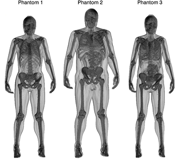
Figure 1. Volume renderings of the mass density distribution of phantom 1, 2 and 3, illustrating the different body sizes and anatomical features.
Download figure:
Standard image High-resolution image2.2. Patient data
Patient time-activity data was acquired from 10 patients after their first therapy cycle with 177Lu-(DOTA0,Tyr3)-Octreotate (DOTATATE). The treatment was performed with an intravenous infusion of 7.4 GBq in 100 mL saline by intravenous infusion during 30 min, in combination with a simultaneous co-infusion of 2000 mL amino-acid solution (Vamin 14 g N L−1 electrolyte-free; Fresenius Kabi). The specific activity of the radiopharmaceutical was approximately 40 MBq μg−1. The imaging protocol consisted of conjugate-view whole-body (WB) planar scans at 1, 24, 96 and 168 h post-infusion (p.i.), including a CT scout image for attenuation correction, as well as a quantitative SPECT/CT study performed at 24 h p.i. The camera system used was a Discovery VH SPECT with a Hawkeye CT unit (General Electric). The emission studies were performed using medium-energy general-purpose (MEGP) collimators, and an energy window of 208 keV ± 10%. Planar image activity quantification was performed using a pixel-based implementation of the conjugate-view method (Sjögreen Gleisner and Ljungberg 2012). The SPECT reconstructions were performed using OS-EM (Ordered-Subset Expectation Maximization) with 8 iterations and 10 subsets, including CT-based attenuation correction, model-based scatter correction (Frey and Tsui 1996) and distance-dependent resolution compensation.
Activity concentrations in the kidneys, liver, spleen and tumours at each time-point were determined by a hybrid method, utilizing data from both SPECT and WB images (Garkavij et al 2010). In this method, the organ activity concentration curve is assumed to follow the time-activity curve determined from the WB data. The curve is then normalised to the 24 h p.i. activity concentration measured in the SPECT image. Liver data from two patients were excluded since the normal liver parenchyma could not be reliably delineated in the planar images due to excessive tumour infiltration. In addition, spleen data could not be obtained for one patient due to a prior splenectomy.
The total-body activity was determined from the WB scans. In addition, the activity content in the urinary bladder was determined from the whole-body scan at 1 h p.i. Since none of the included patients voided between the infusion and the first imaging session, the urinary bladder activity provided a measure of the urinary clearance. Faecal activity was estimated in three patients with prominent intestinal activity at 24 h p.i. The activity was calculated from the SPECT/CT image acquired at 24 h, using the CT for intestinal volume-of-interest (VOI) delineation. Time-activity data for plasma, required for reliable model fitting, were not available for the patients treated at our centre. Therefore, published plasma data from a study employing a similar administration protocol (Esser et al 2006) were used.
2.3. Pharmacokinetic modelling
A first-order linear compartment model, shown in figure 2, was developed to simulate typical pharmacokinetics observed in 177Lu-DOTATATE patients. The primary objective was to construct a PK model that could be used for defining time-varying activity distributions in the phantoms, and thereby provide basis for simulation of realistic and representative images. The PK model was constructed as a closed system to force consistency between the time-activity curves for the different organs and the total-body activity curve.

Figure 2. Model for simulation of 177Lu-DOTATEATE pharmacokinetics. The solid boxes represent individual compartments whereas the dashed boxes indicate groups of compartments associated with a specific set of measured data. Plasma data were obtained from literature as it was not available for the patients in this study. Abbreviations used: R.o.b. = remainder-of-body, int. = internalized.
Download figure:
Standard image High-resolution imageThe plasma volume was represented by a single compartment into which the activity was assumed to be infused at a constant rate during 30 min. The rapid clearance of activity from plasma, reported in e.g. (Kwekkeboom et al 2001, Esser et al 2006), could not be attributed to renal elimination alone. It was thus assumed that there is a rapid transfer of activity into the extravascular space. The liver, spleen, tumour and remaining body were therefore each modelled by at least two compartments respectively, where the first compartment represented an extravascular volume with rapid plasma equilibration, while the second compartment represented a slower component of uptake and release, for instance mediated by somatostatin receptor binding. For the tumours, an additional third compartment was included to account for long-term activity retention due to internalization of the radiolabelled peptide (Waser et al 2009). During model development, it was found that release of internalized activity had to be included to get a good fit to tumour data. To avoid the need of explicit modelling of radioactive metabolites, this release was accounted for by modelling the internalisation as a reversible process.
The kidneys were modelled by two compartments, where the first (rapid) represented activity in the renal filtrate, i.e. activity that had accumulated in the kidneys due to glomerular filtration but had not yet been reabsorbed or excreted into the urinary tract. The second compartment (slow) represented the long-term renal activity retention, mainly due to peptide reabsorption in the proximal tubular cells (Melis et al 2005, Rolleman et al 2010). The tubular uptake was thus modelled as a transfer from the first to the second renal compartment, whereas urinary excretion was modelled as transfer from the first renal compartment to the urinary bladder. To achieve a good fit of the model to renal data, for which a long-term (>24 h p.i.) decrease was seen, a biological washout was included from the second renal compartment. The washout was included as a transfer to the plasma compartment. Although physiologically implausible, this approach maintained the total-body activity and bypassed the need to model radioactive metabolites. Furthermore, the choice of target for this transfer had no discernible impact on the model fit.
Hepatobiliary elimination was included in the model, since intestinal activity is of concern in planar-based dosimetry as it overlaps with renal activity in the anterior–posterior (AP) direction (Garkavij et al 2010). A compartment representing hepatocytic uptake and subsequent biliary excretion was therefore included in the model.
Mathematically, the compartment model was described by a system of first-order linear differential equations following:
where  denotes the decay-corrected activity content of compartment i as a function of time t,
  is the transfer rate constant from compartment j to compartment i and N is the number of compartments.
2.4. Pharmacokinetic model input data and fitting
The patient time-activity data were decay corrected to infusion time, normalized to the injected activity, and interpolated to nominal imaging times at 1, 24, 96 and 168 h p.i. Since the aim of this work was to establish typical pharmacokinetics, geometrical-means of the organ activity concentrations and urinary bladder activity at the different time points were calculated. The total-body long-term activity retention was found to be highly dependent on the tumour burden and associated uptake. Therefore, the total-body activity curve was selected from two of the patients that had a total tumour volume comparable to the phantoms. Utilizing blood-activity data (Esser et al 2006) and vascular volume fractions for tumours and organs of interest (Baxter et al 1995, ICRP 2002), contributions from vascular activity to the measured organ activity concentrations at 1 h p.i. were subtracted. For the remaining time-points, this contribution was considered negligible.
The PK model was implemented in SAAM II software for kinetic analysis (v. 1.2, University of Washington). The SAAM II software is a tool for pharmacokinetic modelling with a graphical user interface that facilitates interactive development of compartment models and subsequent curve fitting to experimental data. In this work, SAAM II was used to fit the transfer rate constants of the PK model (figure 2) by a non-linear least square fit to the acquired patient data (tables 2 and 3). Since the dependent variable of the PK model was compartmental activity (decay corrected), volumes were assigned to the various organs to convert the measured activity concentrations to total organ activity. As the organ volumes differed between the phantoms, an individual fit of the model parameters was performed for each phantom. To increase the generalizability of results obtained using these phantoms, it was considered appropriate that at least one of them would differ from the other in terms of renal activity uptake. Therefore, the input renal activity concentration for phantom 3 was increased with 1 standard deviation (SD), as determined from patient data, before fitting.
Table 2. Activity concentration data used for PK model fitting. The activity concentrations measured in patient organs correspond to a sum of several compartments in the PK model, as indicated by the indices. Activity concentrations are normalized to the injected amount and tissue volume and given in units of %IA/L. All data have been corrected for physical decay.
| Time p.i. (h) | Liver (i = 12, 13, 14) | Spleen (i = 5, 6) | Kidneys (i = 9,10) | Tumour (i = 2, 3, 4) | |
|---|---|---|---|---|---|
| Phantom 1, 2 | Phantom 3 | ||||
| 1 | 1.55 | 5.19 | 6.83 | 8.80 | 26.5 |
| 24 | 2.09 | 7.54 | 6.12 | 7.34 | 29.2 |
| 96 | 1.40 | 5.14 | 3.26 | 4.22 | 24.2 |
| 168 | 1.09 | 3.31 | 1.73 | 2.40 | 21.3 |
Table 3. Activity data used for PK model fitting. The activity is normalized to the injected amount and given in units of %IA. The total body data corresponds to the sum of all compartment activities, except from urine and faeces.
| Time p.i. (h) | Total body (i ≠ 11,15) | Plasma (i = 1) | Urine (i = 11) | Faeces (i = 15) |
|---|---|---|---|---|
| 0.7 | 18 | |||
| 1.0 | 82.6 | 18 | 17.4 | |
| 1.5 | 14 | |||
| 4.5 | 6.5 | |||
| 24.0 | 16.2 | 0.5 | 2.3 | |
| 24.5 | 0.15 | |||
| 96.0 | 10.1 | |||
| 168 | 7.3 |
2.5. Phantom implementation
The compartmental activity contents given by the solution to (1), with associated transfer rate constants, could not be used directly for defining the source distribution within the phantoms since there was not a one-to-one match between the compartments and the XCAT phantom structures. For instance, the phantom has two kidneys with defined renal substructures, whereas both kidneys were merged in the PK model.
To model the passage of the radiolabeled peptide through the kidneys and urinary tract of the phantoms, additional compartments were added. The first (rapid) kidney compartment was subdivided into eight compartments representing activity in renal filtrate and urine residing in the left and right renal cortex, medulla, pelvis and ureter, respectively. The second (slow) kidney compartment was subdivided into two compartments, one for each kidney. The values of the additional transfer constants that were introduced were derived from parameter values obtained from the original fit. The renal uptake rate,  , was divided equally between the two kidneys, and the transfer constants governing the transport of activity through the renal parenchyma and renal pelvis were set to maintain the renal transit time, given by
  in the original model. The reabsorption constants in the extended model were rescaled such that the reabsorption fraction, given by the ratio
  in the original model, was maintained.
The full PK model, including the extended renal transport model, was implemented and solved numerically using the fourth-order Runge-Kutta (RK4) algorithm in IDL (v.8.2, Exelis Visual Information Solutions, Boulder, USA), to yield the activity of each compartment as a function of time. The step-size,  , was 0.07 min and the number of samples, n, was 221. The numerical solutions provided time-activity data up to approximately 101 d p.i. corresponding to approximately 15 physical half-lives of 177Lu.
To define the dynamic activity distribution of the phantoms, the time-activity curves for each structure was calculated as a weighted sum of compartmental activities according to:
where  is the activity in phantom structure q at time
  and
and  is the fraction of activity in compartment i localized in structure q. For the spatial activity distribution to be consistent with the PK model, the total activity in the phantom should equate the total activity of all compartments at all points in time, i.e.
  , where M is the number of phantom structures (see table 1). The factors
  were assigned to obtain the desired anatomical distribution of each compartment, while explicitly ensuring that
  . Most compartments were associated with a single phantom structure by setting
  equal to one for that compartment-phantom structure pair. The plasma compartment (i = 1) was distributed in accordance with the vascular fractions of the phantom structures,
  , i.e.
  where
where  is the total-body vascular volume given by
  . The vascular fraction
  of phantom structure q was defined as
  where
where  and
and  is the vascular volume and total volume of phantom structure q, respectively. For the major structures, vascular fractions were derived from reference data on organ mass, mass density and total and regional blood volumes from ICRP publication 89 (ICRP 2002). Tumour data were obtained from Baxter et al (1995). For the remaining structures the vascular fraction was assumed to be 0.05.
The activity in the two compartments representing the 'remainder-of-body' were assigned to the set of phantom structures that were not associated with a specific compartment in the PK model. Since these compartments represented extravascular localization, the structures containing only air (e.g. the lung airway tree) or blood (e.g. arteries and veins) were excluded. The brain was also excluded from this set of structures due to the poor permeability of somatostatin analogues through the blood-brain barrier (Haldemann et al 1995).
The compartments representing the long-term renal uptake (kidney slow) were associated with both the cortex and medulla since it has been shown that the cortex-to-medulla activity ratio 2–4 d after administration is approximately 70/30 (de Jong et al 2004, Konijnenberg et al 2007). Given that the renal cortex comprises approximately 70% of the total renal volume, the activity in these compartments was distributed in accordance with the fractional volumes of the renal substructures for each phantom. The inhomogeneous activity distribution within the renal substructures reported by de Jong et al (2004) would require a partition of the renal substructures in the XCAT phantom and was therefore not considered.
Elimination of activity from the body by urinary and faecal excretion was accounted for by setting the activity content to zero for the urinary bladder and the intestinal contents every fourth and twenty-fourth hour, respectively.
2.6. Calculation of absorbed dose reference values
The mean absorbed dose rate R to a phantom target structure q was calculated according to
where  denotes the activity located in source organ s at time
  , λ is the 177Lu decay constant, and
  denotes the S value, i.e. the mean absorbed dose rate contribution to phantom structure q per unit activity in s. The absorbed dose rate functions were numerically integrated to yield the total absorbed dose according to
The S values for all source-target combinations in the three phantoms were calculated using a Monte Carlo program for voxel-based internal dosimetry (Liu et al 2001). The program is essentially a wrapper routine for the EGS4 Monte Carlo code (Nelson et al 1985), but includes calculation of beta spectra, sampling of decay positions and spatial energy deposition scoring as further described in (Ljungberg et al 2003). Cross-sections for lung tissue, soft tissue and bone, normalised to unit density, were generated from the EGS4-related utility code PEGS4. In the simulations, the voxel cross-sections were obtained by multiplying the voxel mass density with the suitable normalised cross-section, i.e. lung tissue (ρ ⩽ 0.8 g cm−3), soft tissue (0.8 g cm−3 > ρ ⩽ 1.2 g cm−3) or bone (ρ ⩾ 1.2 g cm−3). The simulations were performed with a homogeneous activity distribution in each source structure, and the resulting energy deposition in all target structures was scored and subsequently divided with the target region mass. The emission spectra and half-life of 177Lu were obtained from the Nudat2 database provided by the National Nuclear Data Center (NNDC 2014). Electron transport was simulated using the PRESTA (Parameter Reduced Electron-Step Transport Algorithm) (Bielajew and Rogers 1986). The cut-off energies, i.e. the energy at which particle tracking is terminated and the remaining kinetic energy is locally absorbed, was 50 keV and 10 keV for electrons and photons, respectively. Five separate simulation batches, each with 106 particle emissions per source structure, were performed with different random number generator seeds to evaluate the numerical uncertainty. The final S values were taken as the average value of the five batches. The numerical uncertainties of  due to discretisation and truncation were heuristically assessed by halving the step-size with the integration interval fixed, and by doubling the integration interval for a fixed step-size, respectively.
2.7. Application example: virtual patient-specific image-based dosimetry
To exemplify the intended use of the phantoms for method validation and accuracy assessment of image-based dosimetry in 177Lu PRRT, a virtual dosimetry study was performed. This sub-study was designed to mimic a dosimetry method that is readily available in most clinics. It should be noted a more exhaustive study will be undertaken in a separate work, and results presented herein are to be regarded as a clinically relevant example.
2.7.1. Imaging simulations.
Activity distribution maps for the three phantoms were prepared using (2) assuming imaging time-points of 1, 24, 96, and 168 h p.i. Acquisitions were simulated using the Monte Carlo code SIMIND (Ljungberg and Strand 1989). The targeted detector system was the Discovery NM/CT 670 system (General Electric) equipped with MEGP collimators, and using an energy window of 208 keV ± 7.5%. Simulated images consisted of whole-body anterior and posterior scans with acquisition durations of 10 min for the image at 1 h, and 20 min for 24, 96 and 168 h, respectively. A SPECT study at 24 h p.i., consisting of 60 projections over 360°, was also simulated. The resulting low-noise image data were re-normalized to represent the simulated image acquisition time of 45 s per projection, and the total amount of activity remaining in the phantom taking both the pharmacokinetics and physical decay of 177Lu (T1/2 = 6.647 d (NNDC 2014)) into account. The pixel values were then replaced by random deviates drawn from a Poisson distribution using the re-normalized pixel values as the mean values. The simulated studies were exported to the clinically used implementation of LundADose, a software package for 2D/3D dosimetry developed at our institution (Sjögreen et al 2002, Ljungberg et al 2003).
2.7.2. Image-based dosimetry calculations.
The methods used for quantitative SPECT reconstruction and planar image quantification of the simulated studies were the same as used for the patient studies (section 2.2). However, the required attenuation maps that were derived from patient CT data in real studies, were instead calculated by mapping the true mass-density distribution of the phantoms to linear attenuation coefficients at 208 keV (Berger and Hubbell 1987). The CT scout images used for planar attenuation correction in the pixel-based conjugate-view method (Sjögreen Gleisner and Ljungberg 2012) were obtained by projecting the 3D attenuation maps onto the coronal plane.
The reconstructed SPECT images were rescaled with the camera system sensitivity and voxel volume to obtain images in units of MBq mL−1. Activity concentrations in the kidneys, liver, spleen and tumours were acquired in small single-slice VOIs to minimise the impact of the partial volume effect (PVE). Rather than using the specific values for the phantom organs to calculate the absorbed doses, S values were obtained from OLINDA (Vanderbilt University, Nashville, Tennessee, USA) (Stabin et al 2005), using the adult female model for the kidneys, liver and spleen; and using the spherical model of appropriate size for each of the tumours. This approach was chosen in order to mimic a real-world scenario where the patient S values are unknown and where Monte Carlo programs for explicit radiation transport calculations are unavailable. One common approach in 177Lu dosimetry is to assume negligible cross-dose contributions from other source organs (Sandström et al 2013). This assumption is reasonable for organs with high uptake given that the 177Lu emission spectrum is dominated by short-range beta particles (maximum range ~2 mm). Using this approximation, the absorbed dose rate estimate  at 24 h p.i. was calculated according to

where  is the SPECT-based activity concentration estimate,
  is the OLINDA self-dose S value, m is the mass of the target organ in the OLINDA model, and ρ is the mass density of the target organ, assumed to be 1.06 g mL−1.
Time-activity values for the organs of interest were determined from the planar images, by delineating region-of-interests and correcting for activity in background and overlapping tissues. The absorbed-dose rate at 1, 96 and 168 h was then calculated as the SPECT-derived absorbed dose-rate 24 h p.i. multiplied with the relative organ activity for each time-point, as determined from the planar image data. A mono-exponential curve was fitted (Wehrmann et al 2007, Bodei et al 2008, Sandström et al 2013), and the absorbed dose calculated by analytical integration.
The whole-body absorbed dose was calculated by fitting and integrating a bi-exponential function (Wehrmann et al 2007) to the total-body activity values determined from the quantitative whole-body scans, and multiplying the cumulated activity with the OLINDA S value rescaled linearly to the phantom mass.
3. Results
3.1. Patient data and phantom pharmacokinetics
The patient dataset used for fitting the PK model parameters (figure 2) are summarized in tables 2 and 3. Measured activity concentrations in kidneys, liver and spleen for the individual patients are shown in figure 3, together with the resulting curves for the three phantoms according to (2). Note that the kidney curves are averaged of the renal cortex and medulla. The concentration of the left and right kidney differ since they have different volumes in all phantoms and were assigned equal uptake rate constants. In addition, the renal activity concentration for phantom 3 is higher than for 1 and 2 as the input dataset was chosen as 1 SD above the mean concentration (table 2). For the other organs, the time-activity curves are virtually identical. It can be noted there is a good agreement between patient and phantom data and that the pharmacokinetics for normal organs are reasonably consistent between patients. It should however be pointed out that the total tumour volume of the phantoms is small relative to the tumour volume of the patients. Since the long-term whole-body activity retention is mainly determined by the tumour burden and associated uptake, the whole-body activity of the phantoms shown in figure 3 should not be considered representative of patients with high tumour burden.

Figure 3. Activity concentration data for the kidneys (n = 10), liver (n = 8), spleen (n = 9), tumour (n = 10) and total body activity (n = 2), decay corrected and normalized to the injected activity of each patient at 1, 24, 96 and 168 h p.i. Thick lines show the calculated quantities for phantoms 1, 2 and 3. The thin dashed lines have been included to visualize the pharmacokinetics for individual patients. The phantom data for liver, tumour and whole-body coincides. The prominent initial peak in the kidney data is a result of the renal blood clearance of 177Lu-DOTATATE resulting in a rapid increase and subsequent decrease of activity in the renal filtrate, as shown in figure 4.
Download figure:
Standard image High-resolution imageThe prominent initial peak in the kidney time-activity data is mainly caused by activity that is in the process of being eliminated through renal filtration, as illustrated in figure 4. Approximately 17% of the activity is located in the urinary bladder one hour after the start of infusion and has thus passed through the kidneys. The height of the peak is dependent on the renal transit time,  , which was determined from the model fitting and found to be in the range 5–10 min for the three phantoms. The initial, smaller, peaks for the other organs are a result of vascular and interstitial activity which is rapidly cleared after the end of infusion. The activity concentrations in the renal cortex and medulla are obtained following the extended renal transport model, as described in section 2.5.

Figure 4. Left: modelled contributions from different compartments to the total renal activity (phantom 1, left kidney). Initially, the main contribution is from renal filtrate and to a lesser extent from vascular activity. The reabsorbed activity retained in the proximal tubules becomes dominant approximately 2–3 h after the start of injection. Right: activity concentrations in the renal cortex and medulla as a function of time.
Download figure:
Standard image High-resolution image3.2. Absorbed dose reference values
The reference values of absorbed dose to the kidneys and renal substructures, liver, spleen tumours and whole-body are given in table 4, assuming a standard activity administration of 7.4 GBq. The mean absorbed doses to the phantom kidneys are in the range 3.05–4.78 Gy, with an expected variation due to the different activity concentration curves, illustrated in figure 3. The mean absorbed dose to the spleen is higher, approximately 5.2 Gy; and for the liver, approximately 1.7 Gy. The tumour absorbed doses are between 26.1–26.9 Gy. The small variation indicates that differences in target volume has minor impact on the absorbed fraction of radiation energy from 177Lu, and that irradiation from activity in other organs is negligible.
Table 4. Absorbed dose (Gy) per 7.4 GBq administered activity for selected phantom structures.
| Phantom 1 | Phantom 2 | Phantom 3 | |
|---|---|---|---|
| Left kidney | |||
| Cortex | 3.44 | 2.98 | 4.03 |
| Medulla | 3.71 | 3.19 | 4.34 |
| Whole | 3.51 | 3.05 | 4.13 |
| Right kidney | |||
| Cortex | 3.36 | 3.93 | 4.68 |
| Medulla | 3.71 | 4.28 | 4.96 |
| Whole | 3.44 | 4.02 | 4.78 |
| Liver | 1.66 | 1.69 | 1.68 |
| Spleen | 5.20 | 5.23 | 5.26 |
| Tumours | |||
| Tumour 1 | 26.58 | 26.89 | 26.94 |
| Tumour 2 | 26.14 | 26.57 | 26.41 |
| Tumour 3 | 26.66 | 26.36 | — |
| Whole-body | 0.25 | 0.17 | 0.28 |
The fractional uncertainties of the reference values due to the Monte Carlo statistics in the EGS4 calculations are in the order of 0.01%. The step-size and integration interval was also found acceptable, with results changing less than 0.1% in the numerical testing described in section 2.6. The combined numerical uncertainty was thus in the order of 0.1%.
3.3. Application example: virtual patient-specific image-based dosimetry
The simulated SPECT studies for the three phantoms corresponding to 24 h p.i. are shown in figure 5, illustrating the different anatomical features of the phantoms as well as the drawback of planar imaging due to overlapping activity in the AP direction. The sequence of WB planar images are shown for phantom 3 in figure 6, also including corresponding images of one patient to enable visual comparison.
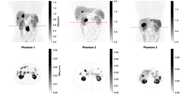
Figure 5. Simulated SPECT studies corresponding to 24 h after administration of 7.4 GBq 177Lu-DOTATATE. Top row: total intensity projection; bottom row: transversal slice. The position of the transversal slice is indicated by the straight line in the top row image. Activity overlapping the kidneys in the anterior–posterior direction should be noted.
Download figure:
Standard image High-resolution image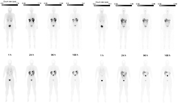
Figure 6. Measured (top row) and simulated (bottom row) whole-body posterior (left) and anterior (right) scintillation camera image data after administration of 7.4 GBq 177Lu-DOTATATE. Each phantom image is shown using the same gray scale as the corresponding patient image to facilitate comparison. Note that there are anatomical differences between this particular patient and phantom and that anatomical resemblance has not been pursued.
Download figure:
Standard image High-resolution image
The absorbed-dose estimates to the kidneys, liver, spleen and tumours are summarized in table 5, as percentage deviations from the corresponding reference value in table 4. The whole-kidney absorbed dose was used as references value for the renal absorbed-dose estimates. In summary, the deviations for all organs and tumours are between −24 and 14%, and for the whole-body absorbed doses between 2 and 4%. The deviations for the tumours are approximately in the same range as the deviations for the organs investigated, and there is no trend of increased accuracy of the absorbed-estimates with increasing tumour volume.
Table 5. Image-based absorbed-dose estimates in percentage (%) of the corresponding reference value. Note that a negative number indicates an underestimation whereas a positive number indicates an overestimation.
| Phantom 1 | Phantom 2 | Phantom 3 | |
|---|---|---|---|
| Left kidney | −13 | −24 | −1 |
| Right kidney | −23 | 4 | 14 |
| Liver | −9 | −9 | −6 |
| Spleen | −6 | −22 | 1 |
| Tumours | |||
| Tumour 1 | 1 | −21 | −16 |
| Tumour 2 | 13 | 13 | −10 |
| Tumour 3 | 10 | 8 | — |
| Whole-body | 2 | 4 | 3 |
4. Discussion
This work describes the development of digital phantoms to be used for method validation and accuracy assessment of image-based dosimetry in radionuclide therapy with 177Lu-DOTATATE. The underlying idea was to create phantoms that have well-defined dosimetric reference values, and that yield realistic image data when used in simulations of scintillation-camera imaging. The dosimetric estimates derived from processing of simulated image data can hence be compared to the reference values to study the accuracy of image-based dosimetry both in terms of trueness (absence of bias) and precision (Menditto et al 2007). In order for such studies to hold merit, it is essential to have accurate and clinically relevant models for the scintillation camera and imaging process, the patient geometry, and the pharmacokinetics of the radiopharmaceutical. To this end, we used a well-validated Monte Carlo code for the imaging simulations, state-of-the-art digital phantoms, and also defined the pharmacokinetic properties by a model fit without explicit assumptions on the shape of the organ time-activity curves. Using this approach, it was possible to generate realistic image data (figures 5 and 6) that captures many of the important features and effects that may deteriorate the accuracy of image-based absorbed-dose estimates.
Since the main focus of this work was to characterise and model the pharmacokinetics of 177Lu-DOTATATE for dosimetry purposes, the PK model (figure 2) with its approximations and possible limitations needs to be further addressed. The radiochemical state and biological processes responsible for the observed spatial redistribution of activity is likely to change with time after injection. Given the limited amount of available input data and the additional model parameters that would be required, we did not include effects of receptor-mediated saturable uptake, protein degradation and formation of radioactive metabolites (Kletting et al 2012). Hence, the physiological interpretation and general applicability of the PK model should not be overstated. However, the compartment model constitutes a closed system where all of the injected activity can be accounted for, thus producing individual organ activities that are consistent with the whole-body activity. This method also assures a physiological plausibility in a few important aspects, e.g. that all activity which is excreted into the urinary bladder passes through the kidneys, thereby producing the initial peak in the renal time-activity curve (figure 4) which may influence estimates of renal absorbed dose if the first imaging session is performed within the first few hours p.i.
Considering that the calculation of the phantom time-activity curves involved several steps after fitting of the original model, the final time-activity curves were verified by comparison to data from the individual patients (figure 3). There was in general a good agreement for all modelled organs and the phantom time-activity curves were found to be representative of the patient group during the time interval investigated. The high inter-patient variability with regards to tumour uptake should be however be noted. This variability is likely in part explained by a true variation between patients, but also by the uncertainty of the time-activity curve estimated using the hybrid planar/SPECT method. The limitations of planar image data, used for assessment of the curve shape, are believed to have a particularly large impact for tumours, being comparably small and often surrounded by organs with different biokinetics, such as the liver. The resulting time-activity curves are thus sensitive to small changes in the ROI delineation and to the effect of surrounding and superimposed activity. Consequently, the outliers in the tumour uptake at 1 h p.i. (figure 3) are probably a manifestation of measurement uncertainty rather than a true deviation in uptake. The outliers were not excluded, but their influence was supressed by using the geometrical mean for calculation of the datasets to which the model was fitted (tables 2 and 3).
It should also be noted that the total-body time-activity curves are based on only two patients with a small tumour burden. Furthermore, patient data was only available up to 168 h p.i., meaning that the phantom curves are extrapolations of the model that have not been verified by measurements. It could be argued that the major part of the absorbed dose is delivered within the first week p.i. and therefore that any discrepancies between the phantoms and typical patients after this time are of less importance. While this is true for the kidneys, the long-term retention of activity in tumours increases the importance of representative tumour curves also for t > 168 h. Thus, any results obtained using these phantoms should be interpreted with this limitation in mind.
The absorbed dose reference values are also associated with uncertainties and should therefore in principle not be considered as true values, as they depend on the adopted emission spectrum and the Monte Carlo code used. The EGS4 simulations used for calculation of S values were benchmarked by comparing calculated absorbed fractions for voxelized spheres with mass between 4 g and 4 kg against corresponding values from OLINDA (Stabin et al 2005). The deviations from the OLINDA values were not higher than 1% for any of the investigated geometries (data not shown) which gives an indication of the uncertainty that can be expected.
Considering that some suggested dose limits in PRRT have been specified in terms of kidney BED rather than the absorbed dose (Bodei et al 2008), we have also implemented a numerical method for BED calculations (Gustafsson et al 2013) that enables calculation of BED reference values to the phantom structures. However, such values would only be valid for the assumed radiobiological model and associated parameters. These calculations would thus require a thorough investigation of appropriate radiobiological parameters, which was considered to be beyond the scope of this work.
To illustrate the intended use of the phantoms, we performed a virtual image-based dosimetry study. The dosimetry protocol was designed to be clinically relevant and generally applicable with regards both to the number and temporal distribution of imaging sessions, as well as to the method for absorbed dose calculations. Thus, we simulated imaging at four time-points with the first week after administration, and calculated the organ absorbed doses based on OLINDA S values, assuming local energy deposition (equation (5)), and neglecting cross-dose contributions as commonly done in practice for 177Lu (Sandström et al 2013). The results obtained in this study indicates that we could, using this dosimetry protocol, expect that mean absorbed doses to patient organs and tumours are correct within approximately 25%, and that the whole-body absorbed dose is correct within approximately 5%. The absorbed-dose estimates where equally accurate for the tumours as for the organs, which was unexpected since the PVE is known to deteriorate the quantitative accuracy for small objects. These results needs to be further verified, partly due to the limitations noted above, but also since the accuracy of the estimates did not decrease with decreasing tumour volume. This result may partly be explained by inconsistent VOI definitions between the different tumours, in combination with overestimated voxel values near the tumour boundaries caused by the Gibbs phenomenon, in turn a result from resolution modelling in the SPECT reconstruction. We do however consider the results from this investigation to be preliminary, as there are several important sources of uncertainties that were not addressed. In this work, the main purpose of the virtual dosimetry study was to verify that there was a reasonable agreement between image-based absorbed-dose estimates and their corresponding reference values. A more thorough study is however currently undertaken in a parallel work, using the phantoms presented herein.
5. Conclusion
Three digital phantoms for method validation and accuracy assessment of image-based dosimetry in 177Lu PRRT have been developed. The phantoms have been provided pharmacokinetic properties that are consistent with 177Lu-DOTATATE patients, based on quantitative scintillation camera measurements and literature data. Reference values, i.e. values that serves as the golden standard, of the mean absorbed dose to the whole-body, kidneys, liver, spleen, tumours of the phantoms have been calculated. In combination with accurate scintillation camera imaging models, realistic image data can be generated, thus enabling image-based dosimetry on realistic virtual patients where the true absorbed dose is known. An initial study showed that image-based estimates of the mean absorbed dose to the organs and tumours, using a clinically relevant dosimetry protocol, were within 25% of their corresponding reference values. The phantoms are expected to be a useful tool to further study and optimise the performance of patient-specific dosimetry methods in 177Lu PRRT, and will be made available upon request to the authors.
Acknowledgments
This work was supported in part by the Swedish Research Council (grant No. 621-2014-6187), the Berta Kamprad Foundation, the Gunnar Nilsson Cancer Foundation and the Swedish Cancer Foundation.