

Abstract
A random walk model for intra-fraction motion has been proposed, where at each step the prostate moves a small amount from its current position in a random direction. Online tracking data from perineal ultrasound is used to validate or reject this model against alternatives. Intra-fraction motion of a prostate was recorded by 4D ultrasound (Elekta Clarity system) during 84 fractions of external beam radiotherapy of six patients. In total, the center of the prostate was tracked for 8 h in intervals of 4 s. Maximum likelihood model parameters were fitted to the data. The null hypothesis of a random walk was tested with the Dickey–Fuller test. The null hypothesis of stationarity was tested by the Kwiatkowski–Phillips–Schmidt–Shin test. The increase of variance in prostate position over time and the variability in motility between fractions were analyzed. Intra-fraction motion of the prostate was best described as a stochastic process with an auto-correlation coefficient of ρ = 0.92 ± 0.13. The random walk hypothesis (ρ = 1) could not be rejected (p = 0.27). The static noise hypothesis (ρ = 0) was rejected (p < 0.001). The Dickey–Fuller test rejected the null hypothesis ρ = 1 in 25% to 32% of cases. On average, the Kwiatkowski–Phillips–Schmidt–Shin test rejected the null hypothesis ρ = 0 with a probability of 93% to 96%. The variance in prostate position increased linearly over time (r2 = 0.9 ± 0.1). Variance kept increasing and did not settle at a maximum as would be expected from a stationary process. There was substantial variability in motility between fractions and patients with maximum aberrations from isocenter ranging from 0.5 mm to over 10 mm in one patient alone. In conclusion, evidence strongly suggests that intra-fraction motion of the prostate is a random walk and neither static (like inter-fraction setup errors) nor stationary (like a cyclic motion such as breathing, for example). The prostate tends to drift away from the isocenter during a fraction, and this variance increases with time, such that shorter fractions are beneficial to the problem of intra-fraction motion. As a consequence, fixed safety margins (which would over-compensate at the beginning and under-compensate at the end of a fraction) cannot optimally account for intra-fraction motion. Instead, online tracking and position correction on-the-fly should be considered as the preferred approach to counter intra-fraction motion.
Export citation and abstract BibTeX RIS
1. Introduction
Intra-fraction motion of the prostate can be a limiting factor to the quality of delivery of external beam radiotherapy. The systematic component of this motion can be substantial for many patients (Mutanga et al 2012) and affects the dose delivered to the tumor and to the surrounding tissue (Yu et al 1998, Nederveen et al 2002, Waghorn et al 2010, Reggiori et al 2011). Like inter-fraction motion, it can be modeled in terms of systematic and random errors to determine an additional margin (Huang et al 2012). Unlike inter-fraction motion, however, prostate displacement tends to increase over time (Bittner et al 2010, Kron et al 2010, Mutanga et al 2012). Hence a fixed margin over-compensates at the beginning of a fraction (directly after correction for inter-fraction motion when the prostate is still close to the isocenter) but under-compensates at the end of a fraction (after the prostate had time to wander off its initial position). A more advanced approach is to track the motion of the prostate online and to correct the table position whenever the displacement becomes too large, see e.g. figure 1 in Litzenberg et al (2012).
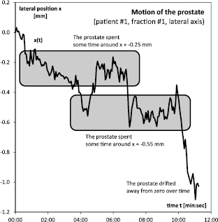
Figure 1. The lateral movement x(t) of the prostate during the first fraction.
Download figure:
Standard image High-resolution imageIn our previous paper (Ballhausen et al 2013) we suggested that the intra-fraction motion of the prostate may be modeled in terms of a time-dependent 'random walk'. In such a model, it is not the position of the prostate that follows a random distribution (which would be described by some constant sigmas), but it is the increments in position between one point in time and the next that follow a random distribution. At each step, the prostate moves from its current position by a tiny amount in a random direction. The result is an erratic motion which when projected onto an axis looks quite like a stock market chart. In particular, a random walk has the required feature that the average displacement of the prostate increases over time, as is observed in intra-fraction time series, see e.g. figure 2 in Bittner et al (2010).
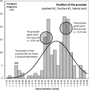
Figure 2. The distribution of the prostate locations was not Gaussian.
Download figure:
Standard image High-resolution imageAssume that the intra-fraction motion of the prostate has been recorded. Its position  is sampled at times
  . Consider the following parameterization of the measurement data:

where ρ describes the correlation between one position and the next, and  is an error term and follows some time-independent random distribution X. There are three possible alternative hypotheses in terms of ρ, and each of them has some implication for external beam radiotherapy:
If  ('static noise' hypothesis), then the position
  is completely independent of the preceding position
  and simply follows X itself. Hence,
  fluctuates around some mean, and the variance of
  is constant. In this case, the duration of a fraction has no impact on the severity of intra-fraction motion. A time-independent margin could be a suitable way to account for intra-fraction motion. Any attempt to tracking and online position correction, on the other hand, would be futile.
If  ('random walk' hypothesis), then the position
  is strongly correlated to the preceding position
  . It is the increments
  that follow X. As a result, the variance of
  increases over time, and the average displacements of the prostate grow larger as the duration of the fraction increases. In this case, online tracking and correction are the preferred option, and failing that, the duration of each fraction should be as short as possible to limit the effect of intra-fraction motion.
If  ('stationary process' hypothesis), the prostate moves freely as long as its displacement is not too large. But there is a tendency to return to its neutral position. Only if ρ is small enough, the variance will eventually approach a maximum during a fraction. Otherwise, the intra-fraction motion will still resemble a random walk, even if ρ is only close to but not equal to one.
In this paper we decide between these hypotheses by comparing hours of tracking data from 4D perineal ultrasound during a series of fractions to the predictions of these alternatives.
2. Materials and methods
Six patients with histologically confirmed adenocarcinoma of the prostate were included in this analysis. All six patients received norm-fractionated external beam radiotherapy in our institution with a cumulative dose ranging from 72 to 76 Gy, depending on the tumor stage. Average age of patients was 65.6 ± 10.1 years (median 65.6 years, range 53.2–77.1 years). Each three fiducial gold markers were implanted in the prostate of four patients, respectively, and image guided IMRT with 6 MV photons was performed for all six patients.
While inter-fraction patient positioning was controlled daily by kV-CBCT, intra-fraction motion of the prostate was tracked during 84 fractions by 4D perineal ultrasound (per patient, 22, 1, 12, 15, 18 and 16 fractions were recorded, respectively). The Clarity ultrasound system was used in combination with an auto-scanning perineal ultra sound probe which provided one image per 0.5 s (Lachaine and Falco 2013). The tracking data was logged at non-equidistant intervals, often several times per second, resulting in 70 573 position readings over a total duration of 9 h and 25 min. For evaluation, tracking data was resampled by averaging over intervals of about 4 s. Invalid data at the beginning and end of each fraction was discarded. Invalid data at the beginning of each fraction was characterized by constant readings or time gaps before regular data logging commenced. Invalid data at the end of each fraction was characterized by sudden movements caused by the motion of the patient or the equipment before data acquisition was stopped. On average, 14% of data per fraction was discarded. After re-binning and clipping, a total of 6901 position readings over a duration of 8 h and 5 min entered evaluation. The choice of the re-binning interval and the choice of clipping were made ex ante and blind to the results.
For the first fraction and the lateral axis, the position of the prostate was plotted as a function of time (figure 1). Both the distribution of the position of the prostate and the distribution of the changes in prostate position were plotted as histograms (figures 2 and 3).

Figure 3. The distribution of increments in prostate position was Gaussian.
Download figure:
Standard image High-resolution imageThe complete data was then analyzed separately for each fraction, and separately along the lateral, longitudinal and vertical axis. For each of the 84 (fractions) × 3 (axes) = 252 trajectories, the model  was fitted to the data. In particular, the maximum likelihood estimator (MLE)
  was calculated from ordinary least-squares (OLS) linear regression of
  against
  . A scatter plot of
  against
  for the first fraction and lateral axis was shown as an example in figure 4, together with the line of best fit with slope
  . The average
  and its error were calculated for the total of 252 trajectories, and separately for each 84 trajectories along each of the three axes (figure 5).

Figure 4. Any two consecutive prostate positions were strongly correlated. The MLE for the correlation coefficient was consistent with one, as predicted by the random walk model.
Download figure:
Standard image High-resolution image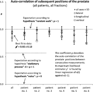
Figure 5. Across all patients and fractions, the correlation of any two consecutive prostate positions was consistent with unity, as predicted by the random walk model.
Download figure:
Standard image High-resolution imageNext, the model was extended to account for a possible offset α (or equivalently, an intercept  ) and for a possible linear time trend
  :
:  . This is the model of Dickey and Fuller (DF) (Dickey 1976, Dickey and Fuller 1979, Fuller 1996). In addition to
  (as above, DF model without intercept or trend,
  ), a MLE
  was calculated from an OLS linear regression of
  against 1, t, and
  (full DF model with intercept and trend). Similarly, a MLE
  was calculated from an OLS linear regression of
  against 1 and
  (DF model with intercept only,
  ). The distribution of these three estimators was plotted as a histogram (figure 6). The Dickey–Fuller test was then employed to test the null hypothesis
  . The one-tailed test statistics
  ,
,  and
and  were compared to the tables given in Dickey (1976). By linear interpolation of these tables, the respective probability was calculated. The null hypothesis
  was rejected if and only if the respective probability was equal to or less than 5% (figure 7).
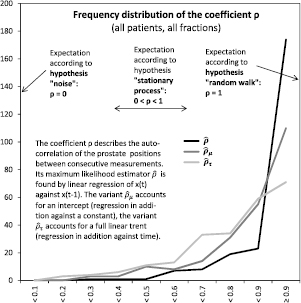
Figure 6. Across all patients and fractions, the correlation coefficient was most frequently above 0.9, even when accounting for possible offsets and linear trends.
Download figure:
Standard image High-resolution image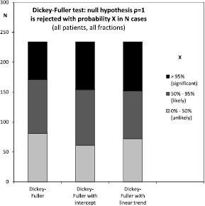
Figure 7. Across all patients and fractions, the Dickey–Fuller test significantly rejected a correlation coefficient of exactly one in about one third of cases.
Download figure:
Standard image High-resolution imageTo test the opposite null hypothesis, the model of Kwiatkowski, Phillips, Schmidt and Shin (KPSS) (Kwiatkowski et al 1992) was employed. Here, the stochastic process is described in terms of a deterministic trend  , a noise or term
  , and a random walk
  :
:  where
where  denotes the intercept, and the random walk is parameterized as
  where the increments
  are independent and identically distributed with mean zero and variance
  . This corresponds to a situation where
  , and the null hypothesis
  states that there is no random walk. Test statistics
  (for
(for  ) and
) and  (for
(for  ) were calculated as in Kwiatkowski et al (1992). The resulting values were compared to the upper tail critical values given there for the asymptotic case
  . By linear interpolation of these tables, the respective probability was calculated. The null hypothesis
  was rejected if and only if the respective probability was equal to or less than 5% (figure 8). To distinguish between the alternatives
  (random walk) and
  (stationary process), the variance of the prostate position was plotted as a function of time (figures 9 and 10). Here, the variance at time t was defined as the variance of the prostate locations at that time t between all recorded fractions. The ex-post observed divergence of the recorded trajectories is thus an empirical measure of the ex-ante uncertainty of the prostate position that increases over time. Finally, the average and maximum distance that the prostate traveled per fraction was analyzed for inter-fraction variability (figure 11) and inter-patient variability (figure 12).

Figure 8. Across all patients and fractions, the KPSS test significantly (>95%) or at least very likely (>80%) rejected the hypothesis, that there is no element of a random walk.
Download figure:
Standard image High-resolution image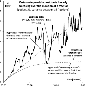
Figure 9. The variance of the prostate position increased over time and was consistent with a linearly increasing variance as predicted by the random walk model. There was no flattening over time observed, as would be predicted for a stationary process with a correlation coefficient smaller than one.
Download figure:
Standard image High-resolution image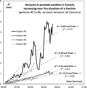
Figure 10. The variance of the prostate position linearly increased over time for all patients (for patient #1 see figure 9; patient #2 was omitted as only a single fraction was recorded).
Download figure:
Standard image High-resolution image
Figure 11. Inter-fraction variability: the maximum distance from the isocenter that the prostate traveled during any given fraction could be as small as 0.5 mm or over 10 mm.
Download figure:
Standard image High-resolution image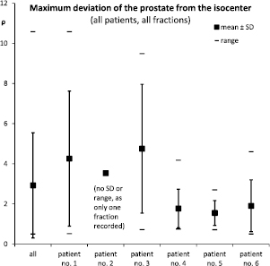
Figure 12. Inter-patient variability: the maximum distance from the isocenter that the prostate traveled during any fraction could be below 3 mm in one patient, and over 10 mm in another.
Download figure:
Standard image High-resolution image
3. Results
For illustration, consider the first patient. During the first fraction, over the duration of 11 min and 14 s, the prostate moved about 1 mm off its initial position in lateral direction, see figure 1. This motion was not linear, however. The prostate moved back and forth in an erratic manner and in total covered a distance that was greater than the net shift at the end of the fraction. Due to this erratic movement, the prostate spent more time in certain areas than in others: during about 90% of time the prostate was within ±0.1 mm of either −0.25 and −0.55 mm, a disjoint pair of areas that covered only about 40% of the overall shift. This can be readily seen in the according histogram, figure 2. There were two spikes around −0.25 and −0.55 mm, but little structure else. In particular, the distribution of prostate positions  could not be fitted by a Gaussian. By contrast, the increments
  shown in figure 3 were indeed Gaussian distributed with mean
  and standard deviation
  . This was in line with the random walk model
  where
where  . In fact, a MLE
  was found by linear regression of
  against
  , see figure 4.
Across all patients and all fractions, the same MLE  was found to be 0.92 on average with a standard deviation of 0.13, see figure 5. Assuming 0.13 as the standard deviation under all hypotheses, the Neyman–Pearson likelihood ratio between the alternatives
  and
and  is
is  such that the static noise hypothesis was strongly rejected in favor of the random walk hypothesis. The static noise hypothesis was rejected as a null hypothesis per se with
  . The random walk hypothesis could not be rejected as a null hypothesis at
  . Results were quantitatively similar between patients, see figure 5. The random walk hypothesis could not be rejected in any single patient, while the static noise hypothesis had to be rejected in all patients. The correlation coefficient was consistently lower on the vertical axis. This is probably because of gravity which acts to keep the prostate in place along the vertical axis, while it has more leeway in the frontal plane.
The distribution of  is shown in figure 6. Out of 252 samples, 174 or 69% were above 0.9, and 197 or 78% were above 0.8. The figure also shows the two distribution of the alternative estimators
  and
and  from the DF model with intercept respectively with intercept and trend. Figure 7 shows the results from the DF test itself: a random walk without intercept or trend was rejected in 63 or 25% of cases. A random walk with intercept was rejected in 80 or 32% of cases. And a random walk with intercept and trend was rejected in 82 or 33% of cases. Figure 8 shows the results for the KPSS test of the opposite null hypothesis. A model of static noise around an intercept was rejected with 95% confidentiality in 149 or 59% of cases. A model of static noise around a linear trend was rejected with 95% confidentiality in 79 or 31% of cases. However, both models were rejected with at least 80% confidentiality in 100% of cases.
The plot of variance in prostate position over time, see figure 9 for the first patient, shows a linear increase of variance over time as predicted by the random walk model. A linear fit  explains most of the data (
 ). A flattening over time was not observed as would be expected from a stationary process. A constant variance, as would be expected from static noise, could not reasonably be fitted to the data. The results are similar for the other four patients (the patient with only one recorded fraction could not be included in this analysis), see figure 10. In each case variance increased over time, and the relationship was even more linear (r2 = 0.77, 0.97, 0.92 and 0.90, respectively). The quantitative motility of the prostate, however, showed some inter-patient variability (
 0.63, 0.16, 0.12 and 0.33, respectively).
There is both substantial inter-fraction variability and inter-patient variability as regards the overall motion of the prostate. For example, figure 10 shows the average distance of the prostate from the isocenter during any of the 22 fractions applied to the first patient, and the maximum distance travelled. During 11 out of 22 fractions, the prostate did not wander off by more than 2 mm. During the other half of the fractions, however, the prostate wandered off by about 6 mm on average, and up to more than 10 mm in one case. The average distance could be as small as 0.2 mm in one fraction and as large as 4.9 mm in another. And the maximum distance traveled even varied between 0.5 and 10.6 mm. This inter-fraction variability was seen to differing degree in all patients, see figure 11. In patients #1 and #3 the maximum distance traveled was about 4 mm on average with a large spread and a range of up to 10 mm. In patients #4 to #6 the maximum distance traveled was only about 2 mm in comparison with much smaller range and spread.
4. Discussion
Across the six patients included in this study, the evidence is strongly in favor of the random walk as a model for intra-fraction motion of the prostate (Ballhausen et al 2013). The alternative model of static noise is ruled out with certainty. The findings are in line with the findings of other groups such as the increasing variance over time in Mutanga et al (2012), Kron et al (2010), Bittner et al (2010) and Adamson and Wu (2010) and offer an explanation for findings such as the non-Gaussian distribution of the prostate location (Lin et al 2013). The average displacement of the prostate of about 2–3 mm is in agreement with results, e.g. from Mutanga et al (2012), and the observed variability is also in line with results, e.g. from Adamson and Wu (2010).
In particular, variance in prostate position increased linearly with time, a hallmark feature of a random walk, and no flattening of variance was observable within 15 min. Thus, the intra-fraction motion of the prostate is also not stationary, at least not during the typical time span of a fraction. In other words, the increase in variance of the prostate position means that it tends to drifts off the isocenter over time. This has two immediate consequences for radiotherapy:
First, shortening the duration of each individual fraction is beneficial, as it limits the opportunity of the prostate to wander off the isocenter, effectively reducing the impact of intra-fraction motion.
Second, intra-fraction motion is unlike inter-fraction variability. Inter-fraction variability manifests in an approximately Gaussian random distribution of the target position at the beginning of a fraction. The respective standard deviation stems from the systematic and random errors (Palombarini et al 2012) remaining after patient positioning or simply from the setup inaccuracy if target localization cannot be repeated daily (Sveistrup et al 2014). An appropriate margin can be computed from optimal margin recipes given these errors.
Unlike such static inter-fraction uncertainties, intra-fraction variability increases with the duration of the fraction. The random walk model predicts a linear increase of the variance with time, as is seen in the data of this paper and larger studies. An additional (constant) 'intra-fraction margin' is not well-suited to account for such an (increasing) variability. It would over-compensates at the beginning of a fraction (when the target was still close to the isocenter) but under-compensates at the end of a fraction (after the target had time to wander off the isocenter).
Moreover, the amount of intra-fraction motion is very different from fraction to fraction and from patient to patient, see figures 11 and 12. Obviously, no one fixed margin can account for this substantial inter-fraction and inter-patient variability.
Hence, instead of chasing intra-fraction motion within the too rigid framework of constant margins, online tracking and position correction on-the-fly appear as the preferred option to counter intra-fraction motion (Shimizu et al 2014).
5. Conclusion
Evidence strongly suggests that intra-fraction motion of the prostate is a random walk and neither static (like inter-fraction setup errors) nor stationary (like cyclic motion, such as breathing, for example). The prostate tends to drift away from the isocenter during a fraction, and this variance increases with time, such that shorter fractions are beneficial to the problem of intra-fraction motion. Also, there is high variability in the motility between fractions and patients. As a consequence, fixed safety margins cannot optimally account for intra-fraction motion. Instead, online tracking and position correction on-the-fly should be considered as the preferred approach to counter intra-fraction motion.
Acknowledgments
We thank Andrea Beisel, Gabriela Danilkiewicz, Sandra Kohlhauser, Anne Kolberg, Patrick Dominik Thum and Anja Weber for their assistance in data acquisition.
Conflict of Interest
Elekta Germany supports research at the university hospital of the Ludwig-Maximilians-University, chair of professor Belka. Elekta supported various congress presentations by professor Belka and Minglun Li. The other authors did not declare any conflict of interest. Funding for research with the Clarity system has been received from Elekta. Elekta had no influence on the study design, the collection, analysis or interpretation of data, on the writing of the manuscript or the decision to submit the manuscript for publication.