
Abstract
The reconstruction of PET brain data in a PET/MR hybrid scanner is challenging in the absence of transmission sources, where MR images are used for MR-based attenuation correction (MR-AC). The main challenge of MR-AC is to separate bone and air, as neither have a signal in traditional MR images, and to assign the correct linear attenuation coefficient to bone. The ultra-short echo time (UTE) MR sequence was proposed as a basis for MR-AC as this sequence shows a small signal in bone. The purpose of this study was to develop a new clinically feasible MR-AC method with patient specific continuous-valued linear attenuation coefficients in bone that provides accurate reconstructed PET image data.
A total of 164 [18F]FDG PET/MR patients were included in this study, of which 10 were used for training. MR-AC was based on either standard CT (reference), UTE or our method (RESOLUTE). The reconstructed PET images were evaluated in the whole brain, as well as regionally in the brain using a ROI-based analysis. Our method segments air, brain, cerebral spinal fluid, and soft tissue voxels on the unprocessed UTE TE images, and uses a mapping of  values to CT Hounsfield Units (HU) to measure the density in bone voxels.
The average error of our method in the brain was 0.1% and less than 1.2% in any region of the brain. On average 95% of the brain was within ±10% of PETCT, compared to 72% when using UTE.
The proposed method is clinically feasible, reducing both the global and local errors on the reconstructed PET images, as well as limiting the number and extent of the outliers.
Export citation and abstract BibTeX RIS

Content from this work may be used under the terms of the Creative Commons Attribution 3.0 licence. Any further distribution of this work must maintain attribution to the author(s) and the title of the work, journal citation and DOI.
1. Introduction
PET is a powerful and accurate diagnostic imaging method for the assessment of patients in oncology (Hillner et al 2008) and neurology (Heiss 2009). Combined PET/CT has been shown to provide intrinsically aligned functional and anatomical image information in single patient examinations (Beyer et al 2011), while offering the additional advantage of using the CT images for noise-limited attenuation correction (CT-based attenuation correction, CT-AC) of PET (Kinahan et al 1998). However, CT images have limited soft tissue characterization and tissue contrast, which limits the usefulness of PET/CT in neurology applications, thus rendering a separate MR examination a requirement for many indications. The introduction of the combined PET/MR, therefore, has a clear advantage over PET/CT, in particular in the context of neurological diseases. PET/MR is, however, limited by the lack of a direct measurement of photon attenuation to be used for attenuation correction (AC), which CT provides. Commercial PET/MR systems today segment the MR images into three classes (air, lung, and soft tissue) (Schulz et al 2011), or four classes (air, lung, fat, and soft tissue) (Martinez-Möller et al 2009) for MR-AC. Neither segmentation method accounts for bone, effectively assigning the linear attenuation coefficient (LAC) of soft tissue to bony areas. The soft tissue LAC is significantly lower than the LAC of bone, causing the PET values to be underestimated particularly in areas in or near bone. In the brain area, due to the skull, a significant bias is present in the area of the cortex as compared to PET corrected with CT (Catana et al 2010). Of note, this bias is spatially variable being highest in the outer cortical structures, with underestimations of more than 20% (Andersen et al 2014). It is an unfortunate coincidence, that neuroimaging, one of the most promising applications of clinical PET/MR, also is the one area suffering most from the shortcomings of MR-AC.
The ultra-short echo time (UTE) MR sequence (Robson et al 2003) was proposed for MR-AC to account for the bias introduced by ignoring the bone (Catana et al 2010). The UTE sequence consists of a pair of MR images obtained at an ultra-short echo time, where a signal can be obtained in bone, and a later echo time, where the bone signal has fully decayed. The other tissue classes (i.e. soft tissue) are similar in both images (Catana et al 2010). The vendor-provided attenuation map based on segmented UTE images consists of three classes (air, soft tissue, and bone). In this implementation, a single LAC is assigned to bone. While being a clear improvement over the attenuation maps without bone, segmented UTE still suffers from errors in the segmentation, resulting in discontinuities of the skull and misclassification of air/tissue interfaces, e.g. the sinuses (Dickson et al 2014) and skull base (Keller et al 2013). This gives rise to local errors in reconstructed PET activity, as well as a radial bias of the same type as that arising when not accounting for bone (Dickson et al 2014). Due to the limited accuracy of the vendor-provided attenuation maps, considarable interest has arisen in the PET/MR community to provide a more suitable solution.
Existing methods in the literature can be separated mainly into atlas-based approaches, reconstruction based techniques to estimate emission and transmission simultaneously and segmentation-based approaches. The atlas-based approaches often involve co-registration of one or more MR images to a database of patients, followed by a back-warp of the CT image corresponding to the best match (Hofmann et al 2008, Burgos et al 2014, Izquierdo-Garcia et al 2014). These types of methods depend on a strong inter- and intra-subject registration, where misregistration due to outlier patients can introduce PET errors. Furthermore, only data similar to patients in the database can be modeled, excluding patients with e.g. cranial surgery and pediatric patients. The methods based on simultaneous estimation of emission and attenuation are based on a maximum a posteriori approach (Nuyts et al 2013). These types of methods are usually limited by the requirement of time-of-flight information, and are yet to be tested on a larger patient cohort imaged in the brain area. Finally, the segmentation-based approaches involve a segmentation of the anatomical MR images into tissue classes that are each assigned with approximated LACs (Martinez-Moller et al 2009, Keereman et al 2010). Local patient specific information, such as anatomical variation or bone density, is usually better modeled using segmentation-based approaches (Bezrukov et al 2013), however, existing vendor-provided methods only model the tissue classes with fixed LACs, which might not be sufficient. A recent publication (Juttukonda et al 2015) utilizes the UTE images to extract a continuous bone signal for each patient. A similar approach is used here, however, our method deviates in a number of important aspects.
We present a new segmentation-based method for MR-AC of brain PET. As opposed to existing segmentation-based methods, our method is able to measure a continuous value for bone density using the  signal (equation (1), see below) derived from the UTE TE images (Catana et al 2010, Keereman et al 2010), as well as segmenting air, soft tissue, brain and cerebral spinal fluid (CSF) values. We use a low threshold for included bone (
 > 100 s−1), which is lower than that in the literature (Keereman et al 2010, Juttukonda et al 2015). We chose to use the lower threshold to capture the full width of the bone, and avoid discontinuities in the skull, as opposed to existing UTE based segmentation methods (Dickson et al 2014, Juttukonda et al 2015). The low threshold might introduce a bias, as the amount of included bone can be locally overestimated, especially in areas of complex air, bone, and tissue combinations. The challenging areas of the nasal septa, ethmoidal-, frontal sinuses and mastoid process in the skull base are therefore handled separately using regional masks. The purpose of this study was to develop a new clinically feasible MR-AC method with patient specific continuous-valued linear attenuation coefficients in bone that provides accurate reconstructed PET image data throughout the brain. The method is compared in 154 subjects to the vendor-provided segmentation-based method and CT as reference.
2. Materials and methods
Patient studies were performed using a fully-integrated PET/MR system (Siemens Biograph mMR, Siemens Healthcare, Erlangen, Germany) (Delso et al 2011) and, for the purpose of obtaining a reference CT image, on whole-body PET/CT systems (Biograph TruePoint 40/64, Siemens Healthcare) (Jakoby et al 2009).
2.1. Patients
Data sets were selected retrospectively from the complete cohort of patients referred for [18F]FDG PET/MR brain examination with indication of neuro-oncology or dementia. We included 164 consecutive patients that were imaged at our institution between November 2013 and September 2014. Of these, 154 were used for evaluation (mean age [±standard deviation]: 67 years [±13.6], mean weight [±standard deviation]: 73 kg [±14.4], 70 females). The original studies were approved by the local ethics committee and all patients gave informed consent. We excluded patients with metal implants in the skull, such as surgery clips, resulting in signal voids in the brain area. We did not exclude patients with dental implants.
2.2. Imaging protocol
2.2.1. PET.
Patients were injected with a mean of 204 ± 21 MBq [18F]FDG and positioned head-first with their arms down on the fully-integrated PET/MR system. Imaging commenced 52 ± 11 min post injection (min: 39, max: 134 min). Data were acquired over a single bed position of 25.8 cm covering the head and neck for 10 min. For the purpose of this study, the PET data from the PET/MR acquisition were reconstructed offline (E7tools, Siemens Medical Solutions, Knoxville, USA). The PET images were reconstructed with MR-AC using 3D Ordinary Poisson-Ordered Subset Expectation Maximization (OP-OSEM) (four iterations, 21 subsets, 3 mm Gaussian post filtering) on 344 × 344 matrices (2.1 × 2.1 × 2.0 mm3 voxels).
2.2.2. MR.
The scan protocol included UTE with repetition time (TR)/echo time 1 (TE1)/echo time 2 (TE2) = 11.94/0.07/2.46 ms, a flip angle of 10 degrees, reconstructed on 192 × 192 × 192 matrices (1.6 × 1.6 × 1.6 mm3 voxels). For evaluation, we also acquired a Dixon sequence with TR/TE = 3.6/1.23 ms, a flip angle of 10 degrees, reconstructed on 192 × 126 × 128 matrices (2.6 × 2.6 × 3.1 mm3 voxels) and a T1w MPRAGE with TR/TE = 1900/2.44 ms, inversion time = 900 ms, flip angle = 9 degrees, reconstructed on 512 × 512 × 192 matrices (0.5 × 0.5 × 1 mm3 voxels). Additional clinical MRIs were acquired for diagnostic use. The software version (VB20P) was the same in all patients.
2.2.3. CT.
A low dose CT (120 kVp, 36 mAs, 5 mm slice width) was acquired and used as a gold standard MR-AC reference.
2.3. Preprocessing of attenuation maps
Four attenuation maps were created. First, vendor-provided MR-based attenuation maps (MR-ACDIXON and MR-ACUTE) were derived using the DIXON VIBE sequence (Martinez-Möller et al 2009) and the UTE MR sequence (Keereman et al 2010). Next, our proposal for a new attenuation map employing REgion Specific Optimization of continuous Linear valued attenuation coefficients based on UTE (RESOLUTE), introduced below, was constructed.
Finally, for each subject, the CT image was co-registered to the T1w MPRAGE MR image using a 6-parameter rigid alignment procedure (minctracc, McConnell Imaging Center, Montreal, Canada) with normalized mutual information as objective function. The patient bed and head-holder were extracted manually from the CT images using an oval ROI (OsiriX software) applied to each transverse CT slice. The attenuation values were then converted from HU to LACs at 511 keV by using the standard bi-linear scaling approach (Carney et al 2006) as implemented in our PET/CT systems. The co-registered CT attenuation map was substituted into the UTE attenuation file (MR-ACCT) to allow for reconstruction. Due to the limited coverage in the neck region of the acquired CT, we replaced the missing area by the values from MR-ACDIXON. To ensure a fair comparison, this replacement was similarly performed in the remaining attenuation maps (MR-ACUTE and MR-ACRESOLUTE). The resulting PET reconstructions are denoted PETCT, PETDIXON, PETUTE and PETRESOLUTE.
2.4. Construction of the attenuation map RESOLUTE
The attenuation map was based on the following masks segmented on the patients: (1) air, (2) patient volume, (3) bone, (4) brain and CSF. The patient volume represents all voxels inside the patient contour, regardless of the tissue type. The masks were obtained by segmenting the original UTE images with echo times TE1 (UTETE1) and TE2 (UTETE2). The construction of each mask is described in detail below, followed in section 2.4.5 by a combination of the masks to construct the final attenuation map.
Air and bone signals have the same lack of intensity in most MR images. In order to separate these we used the UTE images, which have a signal in bone. In order to be able to compare the intensities of UTETE1 and UTETE2 across patients, we initially normalized the images according to a published method (Delso et al 2014). This was achieved by assuming that the soft tissue cluster can be uniquely identified (figures 1(A) and (B)) and separated from air and bone in the joint histogram of UTETE1 and UTETE2 using k-means clustering with k = 2 (figure 1(C)). The images were scaled such that the mean of the soft tissue cluster always had an arbitrary value of 1000. We denote the normalized images nUTETE1 and nUTETE2, and their sum snUTE.

Figure 1. Histograms of UTETE1 (A) and UTETE2 (B) with clear soft tissue peaks. (C) Joint histogram of UTE echoes after soft tissue cluster scaling so the median of the cluster is located at (1000,1000) arbitrary MR units (black cross). The yellow line indicates the splitting border where the threshold is placed between air (lower left) and soft tissue.
Download figure:
Standard image High-resolution image2.4.1. Air.
The air mask was found by thresholding snUTE at the empirically selected threshold 600, which more than likely represents air voxels.
2.4.2. Patient volume.
The patient volume, denoting every voxel inside the patient contour, was derived from MR-ACUTE and the normalized UTE TE images. The signal voids inside MR-ACUTE were filled by a region growing algorithm, and the resulting map was converted to a binary mask. A mask was also created from the UTE TE images by setting voxels to 1 if snUTE was greater than an arbitrary threshold of 1000, which more than likely represents soft tissue voxels. We considered a voxel to be inside the patient volume if either mask was 1.
2.4.3. Bone.
Investigating the difference between UTETE1 and UTETE2 gives a signal in voxels with bone. Using  as a measure, it is possible to distinguish cortical bone from soft tissue, because of the significant difference in relaxation rate between both tissue types (Keereman et al 2010):

Instead of simply thresholding the  map, as has been proposed (Catana et al 2010, Keereman et al 2010), we here wished to obtain a continuous value related to the bone density. To this end, we aligned the CT to the
  map in 10 patients using non-rigid registration (SPM8; Wellcome Trust Centre for Neuroimaging, University College London, United Kingdom). These patients were not included in the set of 154 patients for the later performance analysis. For each
  and CT voxel pair with CT intensity greater than 50 HU, we located the maximum
  value and CT value in a 5 × 5 neighborhood. To limit the noise from
  we sorted the pairs in bins of size 10 s−1 and calculated the median for each patient in each bin. We then fitted a third order polynomial to the median points in order to obtain a mapping from
  to CT HU values. The median points (±standard deviation to the mean) are shown together with the fitted polynomial in figure 2. Using this mapping, for each new patient we converted the values in the
  map greater than 100 s−1 to CT HU, and from there, scaled the image to LAC (Carney et al 2006). To limit bias we excluded bone from voxels with high likelihood of being soft tissue voxels by thresholding nUTETE2 at 1200, assuming the bone signal had fully decayed in this image.

Figure 2.  versus HU scatter plot with sampled points shown for each patient in gray (n = 10). Every third median bin-value showed with black squares. Standard deviation to the mean value is shown with black error bars. A 3rd order polynomial fit to the median points is shown with the blue line, r2 = 0.93.
Download figure:
Standard image High-resolution image2.4.4. Brain and CSF.
The UTETE2 image of each patient was nonlinearly registered to MNI space using the ICBM 2009a T1-weighted average structural template image by applying a combination of affine and nonlinear registrations (ANTS, PICSL, Philadelphia, PA). The mask of the corresponding ICBM template brain in MNI space was then warped back to the patient and defined the area of the brain. The white matter and gray matter, and the CSF values, were segmented on the T1w MR image using INSECT (Collins et al 1999). We assigned the LACs 0.096 cm−1 to CSF areas (Carney et al 2006), and 0.099 cm−1 to the rest of the brain (Wagenknecht et al 2013). The values were verified by inspecting the brain values in the CT images of the 10 training patients.
2.4.5. Combining the masks.
In order to model the complex areas with mixed air and tissue, we used a regionally varying combination of the masks in the frontal sinus, the nasal septa and ethmoidal sinus, the skull base, and the rest of the patient volume. Each of the region specific areas was located by alignment of the UTETE2 MR image to the ICBM template where the regional masks were originally defined (figures 3(A)–(D)).
2.4.5.1. Frontal sinus.
For the frontal sinus an LAC of 0 cm−1 was assigned for all voxels within the air mask regardless of the  signal. This choice was due to the signal in this area being purely noise (figure 4(A)).
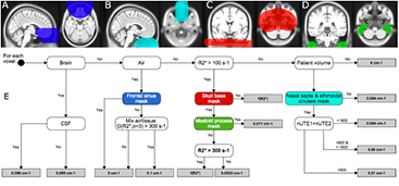
Figure 3. Regional masks (top) and workflow of the algorithm (bottom). (A) illustrates the frontal sinus mask, which limits the amount of bone in the air regions, (B) nasal septa and ethmoidal sinuses, a special segmentation of the mixed tissue regions, (C) skull base, which limits the  signal to include only voxels with high bone density, (D) mastoid process in skull base, which limits the
  bias in the mastoid process by setting voxels to soft tissue values. (E) illustrates the LAC assignment for each pixel. The function G(
 , σ = 3) denotes a 3 mm Gaussian blurring of
  , and f(
 ) denotes the mapping of
  values to LAC. The four regional masks are indicated with colored backgrounds.
Download figure:
Standard image High-resolution image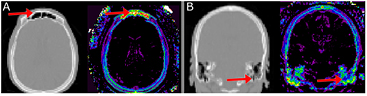
Figure 4. Complex air/tissue interface areas results in noisy  signal in (A) the frontal sinus and (B) the skull base. Left in each is CT, right shows the corresponding
  signal. The masks shown in figures 3(A)–(D) remedy these areas.
Download figure:
Standard image High-resolution image2.4.5.2. Nasal septa and ethmoidal sinuses.
To model the mixed air/tissue area in the nasal septa and ethmoidal sinuses, we assigned 0.01 cm−1 to voxels where snUTE < 800, and 0.06 cm−1 when 800 < snUTE < 1600. This two-value assignment from the UTE images provided a separation of the air filled cavities and the complex thin-wall structure consisting of bone and cartilage.
2.4.5.3. Mastoid process.
Inside the mastoid process in the skull base we assigned a value representing a mix of tissue and bone (0.11 cm−1) to the bony voxels. This was done to limit the impact of the bias in the air/tissue/bone at the skull base near air/tissue interfaces (figure 4(B))
2.4.5.4. Skull base
The mixed air/tissue/bone area in the skull base introduces noise in the  signal for low values. Therefore only voxels with high bone density (
 > 300 s−1) were mapped as bone (figure 2). For the remaining voxels within the skull base mask an LAC of 0.0925 cm−1 was assigned to represent a mix of air, tissue and low-density bone.
In order to model the areas with mixed air and bone signal, all voxels within the classified air mask, except the frontal sinus, containing a  signal greater than 300 s−1, representing dense bone, were assigned an LAC value for mixed air and bone (0.1 cm−1). To avoid introducing
  noise in this region, the signal was blurred with a 3mm Gaussian before thresholding. The rest of the tissue masks were combined hierarchally inside the patient volume mask, in the top down order: CSF > brain > air/tissue mix > air > bone > soft tissue. The LAC for soft tissue was chosen to be 0.094 cm−1 representing mainly skin, muscle and fat (Wagenknecht et al 2013). The thresholds used for the segmentation and the LAC values chosen for the mixed tissue areas were heuristically determined in an iterative manner after first analyzing the corresponding areas in the CT images of the 10 training patients. The optimized LAC values are summarized in table 1. The algorithm is given in detail in figure 3(E). The final attenuation map was blurred with a 4 mm Gaussian filter.
Table 1. Linear attenuation coefficients applied to the tissue interfaces and classes.  represents the mapping of
  to LAC.
| Region | LAC (cm−1) |
|---|---|
| Air | 0 |
| Air/tissue (air weighted, snUTE < 800) | 0.01 |
| Air/tissue (tissue weighted, snUTE 800–1600 | 0.06 |
| Air/low density bone | 0.0925 |
| Soft tissue (skin, muscle, fat) | 0.094 |
| Cerebral spinal fluid | 0.096 |
| Brain | 0.099 |
| Air/bone | 0.1 |
| Tissue/bone | 0.11 |
| Bone |  |
2.5. Image analysis
The analysis was designed to evaluate the accuracy of the continuous bone in the attenuation maps, as well as both global and regional performance in the reconstructed PET images. Each of the metrics is introduced below.
2.5.1. Accuracy of bone.
Dice coefficients were calculated according to equation (2):

where X denotes either the evaluated MR-AC maps UTE or RESOLUTE. The average voxel wise LAC %-difference was calculated in the voxels classified as bone in both CT and the evaluated AC method. This was done to assess the accuracy of the bone segmentation as well as that of the continuous bone measurements.
2.5.2. PET error and common space.
To analyze the result on the PET images, we calculated the voxel-wise %-difference with CT based attenuation as reference:

for all patients, where X denotes Dixon, UTE or RESOLUTE, respectively. In order to compare across all patients, the images were moved into a common space using the non-linear alignment to the ICBM template in MNI space as described above.
2.5.3. Overall PET performance.
To assess the overall performance of the methods, we first computed the averaged whole brain error across all patients using (equation (3)), as well as the images of pixel-wise mean across all patients and displayed them overlaid into the ICBM template to show the distribution of errors spatially. Mean absolute error for the whole brain that disregard the direction of over- and under prediction are included for comparison. We then calculated the joint histograms between PETCT and PETDIXON, PETUTE and PETRESOLUTE, respectively, as well as the histogram of errors for each of the methods. This gave a good overall assessment of the methods.
2.5.4. Regional PET performance.
The voxel-wise fractions of patients having errors greater than ±5% were calculated for each voxel in the brain, and displayed overlaid onto the ICBM template. In practice, this was done for each voxel by counting the number of patients having errors greater than ±5% and dividing by the number of patients. This map can be interpreted as a probability map of errors greater than ±5%. This metric gave an image-based representation of outliers, as well as identified systematic regional bias. The average fraction of the brain having errors greater than ±15%, ±10% and ±5%, respectively, were calculated. To evaluate the regional errors, the mean value of the predefined anatomical ROIs defined on the ICBM template was used. For each of the methods Dixon, UTE, and RESOLUTE, we report the mean and standard deviation across all patients, as well as the maximum patient error.
2.5.5. Effect of the regional masks.
To analyze the effect of the regional masks on the PET performance, we created an additional attenuation map where we disregard the regional masks introduced in figure 3. The effect was assessed using the whole brain error and selected ROI analysis averaged across all 154 patients.
3. Results
3.1. Segmentation and accuracy of bone in the MR-AC maps
The attenuation maps obtained with our method in comparison with the vendor provided UTE and the gold standard CT image are shown in figure 5. Dixon was excluded from this analysis, as the MR-AC map does not contain any bone. The Dice coefficients for the overlapping bone were 0.71 for UTE and 0.81 for RESOLUTE. The averaged %-difference to the LAC in bone voxels in the aligned CT was −16% ± 6% (max: −36%) when using UTEs fixed LAC value for bone. This was reduced to −1% ± 3% (max: −8%) when using RESOLUTE with continuous bone value, suggesting that the  map is indeed able to measure the correct bone density.

Figure 5. Comparison of attenuation maps for a representative subject. MR-ACUTE (A), MR-ACRESOLUTE (B), and MR-ACCT (C) are displayed in 3 orientations (the neck area not covered by the CT has been replaced by the corresponding Dixon voxels in all images). Notice the air segmentation in the nasal septa (blue arrows) and air/bone segmentation in the frontal sinus (red arrows).
Download figure:
Standard image High-resolution image3.2. Overall PET performance
The average error over the full brain was −0.1% (±2.8%), compared to −6.9% (±2.1%) in UTE. The mean absolute error over the full brain was 3.4% (±1.6%), compared to 8.2% (±1.9%) in UTE. The averaged %-difference image from PETCT to PETDIXON, PETUTE and PETRESOLUTE, respectively, is shown in three orientations (figure 6). Notice the error of 10–15% in UTE near the cortex (figure 6(B)). This error is reduced to less than 1% when using RESOLUTE. The results for the averaged joint histograms are shown in figure 7. The values in PETRESOLUTE are closer to PETCT than PETUTE, which is supported by the r2 scores of 0.66 for Dixon, 0.78 for UTE and 0.92 for RESOLUTE. The systematic underestimation compared to PETCT when using Dixon and UTE is significantly reduced when RESOLUTE is applied for MR-AC. A histogram of errors can be seen in supplementary figure 1 (stacks.iop.org/PMB/60/8047/mmedia). We saw an improvement of our method over UTE and Dixon, as the number of voxels greater than ±5% was significantly reduced and the number of voxels around 0% error was increased. The systematic negative bias observed in UTE and DIXON was also considerably reduced.
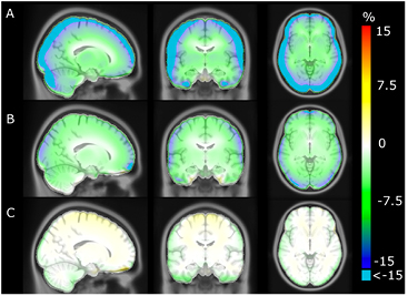
Figure 6. Averaged %-difference images of 154 patients. (A) shows Dixon, (B) UTE and (C) shows RESOLUTE. Notice that errors of less than −15% are clamped to cyan in A and B.
Download figure:
Standard image High-resolution image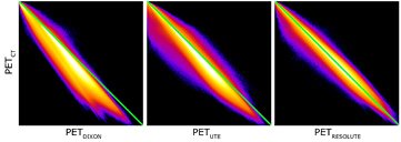
Figure 7. Summed joint histograms of PET values in the brain for all patients. r2 = 0.66/0.78/0.92 for PETDIXON/PETUTE/PETRESOLUTE.
Download figure:
Standard image High-resolution image3.3. Regional PET performance
An image showing the voxel-wise fraction of errors greater than ±5% is presented in figure 8. The probability of having errors greater than ±5% at the cortex is more than 90% when using UTE but only 10–25% when using our method. The probability of an error at the frontal sinus and in the cerebellum is also significantly reduced. Using RESOLUTE, the average fraction of the brain within ±10% and ±5% from PETCT was 95% and 77%, respectively (table 2). In comparison, Dixon/UTE gave 37%/72% within ±10% and 7%/28% within ±5%. The ROI based comparison is presented in figure 9. Using our method, the average error was below −1.2% in all regions of the brain, including the cerebellum, which is often confounded by complex air/tissue interfaces for the regions in the vicinity.
Table 2. Amount of brain being within ±5%, ±10%, and ±15% of the PETCT values. Result is averaged across all 154 patients.
| Region | Within ±5%(±std) | Within ±10%(±std) | Within ±15%(±std) |
|---|---|---|---|
| Dixon | 7.2 ± 5.2 | 36.8 ± 13.6 | 67 ± 15.9 |
| UTE | 28.3 ± 15.6 | 72.2 ± 14.2 | 91.7 ± 6.3 |
| RESOLUTE | 77.3 ± 21.2 | 95 ± 5 | 98.6 ± 1.2 |
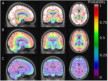
Figure 8. Probability of error greater than ±5% for each voxel. (A) shows Dixon, (B) UTE and (C) shows RESOLUTE.
Download figure:
Standard image High-resolution image
Figure 9. ROI analysis showing averaged mean (colored bars), standard deviation across patients (gray errorbars), and maximum outliers (small colored squares).
Download figure:
Standard image High-resolution image3.4. Effect of the regional masks
An example of the %-difference images for a patient with all the regional masks ignored, compared to application of the masks, is shown in figure 10. The error in the whole brain averaged across all patients was 2.5% (±3.1%) when ignoring all four regional masks. Compared to figure 9, the regions with errors worth noting when ignoring the regional masks were the medulla, the cerebellum, and the frontal cortex with errors of 7.0% (±4.9%), 5.9% (±5.0%), and 2.5% (±3.5%), respectively. The maximum error increased significantly in all regions compared to when applying the masks. Of note, the maximum error in the cerebellum was 22%.
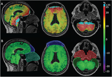
Figure 10. Sample patient shown with %-difference to CT for our method without regional optimization (A) and RESOLUTE with the regional optimization (B). The areas of the regional optimization (see figures 3(A)–(D)) were manually outlined and overlaid. Notice the bias in the skull base and mastoid process causes overestimation in the cerebellum, and the bias from the frontal sinus and failure to segment the air in the nasal septa causes overestimation in the frontal lobe. The error is significantly reduced when using the regional optimization limiting the impact of the bias.
Download figure:
Standard image High-resolution image4. Discussion
In this study we have presented our new attenuation correction method (RESOLUTE) for brain PET/MR hybrid imaging. The only MR sequence used is UTE, and from this we measure the bone density of each patient, and classify voxels as brain, CSF, air and soft tissue using segmentation techniques. Challenging areas of the nasal septa, ethmoidal-, frontal sinuses and mastoid process in the skull base are handled separately using regional masks. The errors in the reconstructed PET data based on our method are small; from a comprehensive quantitative analysis we highlight that the average error in the brain is 0.1%, less than 1.2% in all regions of the brain and on average 95% of the brain voxels are within ±10% of the PET value derived using CT-based AC. The process to create the attenuation map takes 10–15 min on a standard desktop computer, and is fully automatic.
The produced attenuation map looks very similar to that of CT (figure 5), and is a clear improvement over the vendor-provided UTE technique, both with respect to bone density, thickness, and accuracy of bone and air, especially in the frontal sinus area. The average LAC %-difference to CT in bony voxels was 1%, and maximum 8%, suggesting that the  signal is indeed able to measure the patient specific bone density.
Since our method is based on the vendor-provided UTE sequence, we should assess our accuracy of PET reconstruction in the regions where the vendor-provided UTE based attenuation map is known to struggle. This is especially behind the frontal sinus and in the skull base (Keller et al 2013, Dickson et al 2014). In the averaged %-difference images we see how the 8–15% error behind the sinuses and 5–8% error in the cerebellum near the skull base, when using the UTE technique, is significantly reduced when using our method (figures 6 and 9). The improvement of using continuous bone values instead of the fixed value in UTE is clearly demonstrated in figure 8, as the probability of an error greater than ±5% near the skull is reduced from around 90% to 20% when using our method. Our segmentation of the UTE signal and assignment of continuous bone signal also seems to limit the number and extent of the outlier results, as 95% of the brain voxels are within ±10% of PETCT, compared to only 72% when using UTE (table 2).
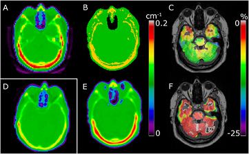
The reduced error due to the use of RESOLUTE AC is caused by several competing effects. Firstly, RESOLUTE segments the large brain region and assigns an LAC value of 0.099 cm−1 that is lower than the vendor-provided value generally used for soft tissue (0.1 cm−1). This affects all regions in the brain. Secondly, the accurate air segmentation affects the regions near air cavities, in particular the frontal sinuses. Finally, PET AC with RESOLUTE benefits from the assignment of continuous bone values. Using a single value for bone (vendor-provided UTE, (Anazodo et al 2014)), or using an incorrect pseudo CT skull value (Burgos et al 2014, Izquierdo-Garcia et al 2014) in the MR-AC map, can in some individuals result in large regional PET errors in the brain close to the skull. This is exemplified in figure 11 where failure to compensate for the high bone density results in errors in the PET image of up to 25% in the cerebellum. Since our method is able to capture and model outlier patients with high density in the skull, this error is reduced.
Figure 11. Sample patient with high bone density. Attenuation map shown for CT (A) and UTE (B) where the fixed bone value causes underestimation of PET uptake in the brain (C) showing Δ%(PETUTE). RESOLUTE (E) is able to measure the bone density, resulting in an improved PET image (F) showing Δ%(PETRESOLUTE). Sample of normal bone density CT image from another patient shown for comparison (D).
Download figure:
Standard image High-resolution image
Results similar to ours were also presented by Burgos et al (2014) and Izquierdo-Garcia et al (2014) using atlas-based approaches that predict CT HU from T1w images, Johansson et al (2014) with a machine learning method based on a mixture of Gaussians using two pairs of UTE images, Navalpakkam et al (2013) with a support vector regression method using Dixon image and a pair of UTE images, and Juttukonda et al (2015) using the  signal to model the individual bone density. The mean error (ME) or mean absolute error (MAE) reported for the full brain region on PET is for Burgos: 0.2%/2.9% (ME/MAE, 41 subjects), Izquierdo-Garcia: −1.2% (ME, 15 subjects), Johansson: 1.9% (ME, 8 subjects) (Larsson et al 2013), Navalpakkam: 2.4% (MAE, 5 subjects), and Juttukonda: 2.6% (MAE, 98 subjects). This should be compared to the results reported here: −0.1%/3.4% (ME/MAE, 154 subjects). Atlas based methods generally have limitations in representing features not present in the database such as morphological changes, missing skull due to surgery and anatomical features such as bone density. Burgos states that bone density information could be added to the method to improve the similarity estimate. The method by Izquierdo-Garcia uses a single atlas and is presumably less robust to variations in gender, age and ethnicity and provides no information on bone density. The method by Johansson is limited by the practical applicability, as it requires multiple pairs of UTE images, as well as the limited accuracy in the nasal septa region due to the large amount of air/tissue interfaces. We address this area specifically. The method by Navalpakkam is yet to be evaluated on a larger patient cohort.
The method by Juttukonda is, similarly to ours, based on prediction of a continuous bone value using the  signal. The method deviates from ours by the threshold for included bone. The authors use a higher threshold (550 s−1) than Keereman et al (500 s−1) (Keereman et al 2010) in order to limit the amount of fat and CSF voxels included in the bone segmentation. We chose the lower threshold of 100 s−1 since the CT values at this threshold are 200–400 HU (figure 2), representing bone, and should therefore be included to capture the full width of the skull and to avoid discontinuities. The bias at the air/tissue interfaces (figure 4) results in an overestimation of PET values when not compensated for, as shown for a sample patient (figure 10). Comparing the %-difference images shows that without the regional masks the error in the cerebellum is up to 25% regionally for this patient. This error is significantly reduced when applying our regional masks. The global mean error across all patients in the cerebellum increases from −0.9% when applying the masks, to 4.7% when ignoring the masks. Juttukonda et al proposes to use the Dixon sequence to account for the bias by segmenting the soft tissue areas where bone is unlikely to occur. We chose not to use the Dixon images due to the possibility of misregistration to UTE, the simplicity of the acquisition sequence, as well as the large voxel size. Using the Dixon images also limits the usability of the method as these have been shown to be confounded by fat–water inversion present in 8% of scans (Ladefoged et al 2014). We instead limit the bias by excluding bone from voxels with high probability of being soft tissue or brain voxels, both segmented using the UTE TE images.
An accurate attenuation map is crucial for obtaining quantitative correct PET images, which is essential for clinical evaluation, especially in the case of tumor staging and treatment response assessment (Wahl et al 2009). We have shown that our method gives very low PET errors, in the range of less than 5–10% dependent on the evaluation method, but have not discussed the requirements for clinical use. Our method has proved to be very robust, as illustrated in the ROI-based analysis, which shows a low mean error across all regions of less than 1.2%, compared to 4–12% using UTE. Of note also, the error in the cerebellum region is significantly decreased from 7% to 0.9%. This is important for the applications using the cerebellum as a reference region, e.g. for normalization of activity (Ishii et al 2001, Yakushev et al 2008, Borghammer et al 2010). The reduced error and low number of outliers indicate that the method could be used in clinical routine. This should be evaluated further addressing clinical reading directly. Our method is, of course, limited by the accuracy of the UTE TE images. Segmentation errors can therefore occur in the case of inhomogeneities or signal voids induced by metal implants. In this work, we have not attempted to correct for this, but propose to use already existing metal artifact correction techniques in combination with our method (Ladefoged et al 2015). The method is also limited by the registration accuracy of the aligned masks for the sinuses and base of the skull. It was not a problem in this study, as we do not rely on very accurate alignment. The purpose of the masks is to locate the air regions, which are usually uniquely identifiable.
Due to the normalization of the UTE images, the applied thresholds were the same for all patients, which removed the need for any user intervention. The normalization and the thresholds were optimized on only 10 patients only used in the training step, and were directly applied to the 154 patients used for evaluation in this study. The values for each tissue class were chosen by inspecting the corresponding CT images of the training patients. The values are comparable to those reported by other authors (Wagenknecht et al 2013).
The fundamental idea of this method is not limited to brain attenuation correction, and is adoptable to a larger patient group. The crude masks are delineated on the ICBM template constructed using adult patients. Similar templates are available from children and various animals, presumably making the method applicable to different types of patients, regardless of gender, age and ethnicity as well as for animal studies. The possibility of adding UTE sequences outside the head would make the  mapping useful for whole-body attenuation correction. The proposed method shows clear improvements over the existing Dixon and UTE techniques. The evaluation of 154 patients demonstrated that the results are representative of the performance of the method, and we are currently using it for clinical evaluation at our institution.
5. Conclusion
We propose an MR-based attenuation correction method (RESOLUTE) for PET derived from hybrid PET/MR brain imaging. The method uses patient specific segmentation of brain and air regions, as well as an assignment of continuous bone. The method makes use of existing vendor-provided UTE images for the segmentation of tissue. The accuracy of the bone segmentation and the ability of measuring the correct bone density are clear from our analysis results. The improvement over the vendor-provided UTE with fixed bone values and regional segmentation errors reducing both the global and local error on the reconstructed PET images, as well as limiting the number and extent of the outliers. Having evaluated the method on a cohort of 154 patients, with a global average error of only 0.1%, an error of less than 1.2% in any region of the brain and on average 95% of the brain within ±10% of the reference, we have demonstrated that RESOLUTE is ready for further clinical evaluation.
Compliance with ethical standards
Conflict of interest. All authors declare no conflict of interest. Ethical approval. All procedures performed in studies involving human participants were in accordance with the ethical standards of the institutional and national research committee and with the 1964 Helsinki declaration and its later amendments or comparable ethical standards. Informed consent. Informed consent was obtained from all individual participants included in the study.
Acknowledgments
The PET/MR system was donated by the John and Birthe Meyer Foundation. We thank Dr Gillings for linguistic corrections.