
Abstract
Objective. Human scalp electroencephalogram (EEG) is widely applied in cognitive neuroscience and clinical studies due to its non-invasiveness and ultra-high time resolution. However, the representativeness of the measured EEG potentials for the underneath neural activities is still a problem under debate. This study aims to investigate systematically how both reference montage and electrodes setup affect the accuracy of EEG potentials. Approach. First, the standard EEG potentials are generated by the forward calculation with a single dipole in the neural source space, for eleven channel numbers (10, 16, 21, 32, 64, 85, 96, 128, 129, 257, 335). Here, the reference is the ideal infinity implicitly determined by forward theory. Then, the standard EEG potentials are transformed to recordings with different references including five mono-polar references (Left earlobe, Fz, Pz, Oz, Cz), and three re-references (linked mastoids (LM), average reference (AR) and reference electrode standardization technique (REST)). Finally, the relative errors between the standard EEG potentials and the transformed ones are evaluated in terms of channel number, scalp regions, electrodes layout, dipole source position and orientation, as well as sensor noise and head model. Main results. Mono-polar reference recordings are usually of large distortions; thus, a re-reference after online mono-polar recording should be adopted in general to mitigate this effect. Among the three re-references, REST is generally superior to AR for all factors compared, and LM performs worst. REST is insensitive to head model perturbation. AR is subject to electrodes coverage and dipole orientation but no close relation with channel number. Significance. These results indicate that REST would be the first choice of re-reference and AR may be an alternative option for high level sensor noise case. Our findings may provide the helpful suggestions on how to obtain the EEG potentials as accurately as possible for cognitive neuroscientists and clinicians.
Export citation and abstract BibTeX RIS

Original content from this work may be used under the terms of the Creative Commons Attribution 3.0 licence. Any further distribution of this work must maintain attribution to the author(s) and the title of the work, journal citation and DOI.
1. Introduction
Since its discovery in 1929, human scalp electroencephalogram (EEG) has been an indispensable tool for brain study due to its sensitivity, non-invasiveness, and high time resolution. Cognitive neuroscientists, clinicians, and engineers have been telling nice stories about utilizing EEG in cognitive psychology, neurology and neuropsychiatry, as well as virtual reality and brain–computer interface, respectively. A successful application of EEG usually depends on signal processing methods, including time-frequency analysis [1] in temporal domain, topography analysis [2, 3] on the scalp surface, and tomography analysis or source analysis [4–6] in the brain. These analyses require the approximation of source model [7], head model, volume conduction model, and most importantly the true scalp EEG recordings.
To obtain true scalp recordings, we need not only to control various environment noises but also to mitigate the distortion effect of a non-zero reference. Principally, EEG potentials are the potential differences between the active electrodes and the reference electrode [8]. During the past decades, people were always pursuing an approximate zero reference electrode so that the active electrodes could locally record the actual time varying potentials. However, it is impossible to find an inactive or a neutral point on the body surface. The choice of reference is still unsolved by a good way resulting in inconsistent usages and endless debate that is so-called 'reference electrode problem'. So far, a rich family of reference montages has been suggested, including online recording references with various mono-polar references in common use, and offline re-references such as linked mastoids (LM) [9], average reference (AR) [10], and reference electrode standardization technique (REST) [11]. Prior studies have shown that the choice of reference may have great impacts on EEG waveforms and power spectra [12–14], and the effectiveness of a reference is affected by various factors, particularly like channel number [11, 15–17].
In current practice, there is a large variation for channel number: the prevalent 10 and 16 channels for clinical use, the high dense arrays from 64 to 256 channels frequently adopted in cognitive neuroscience, even ultrahigh sensor density with more than 300 channels in some studies [18, 19]. However, previous studies on the effect of channel number to re-reference are limited to 21-256. It is definitely necessary to perform a comprehensive evaluation for channel number from 10 to 300 even above. In addition, with channel number increasing, how are these electrodes placed over the head? The international 10-20 placement system typically with 21 channels is the first proposal to standardize the electrodes layout [20]. Then, 10-10 and 10-5 placement systems are the derivatives of 10-20 system with more channels nominated to meet the needs of advanced source imaging techniques [18, 19, 21, 22]. Namely, these systems define more electrode sites as relative head-surface-based positioning rule in addition to the electrodes sites of primary 10-20 system. This series of system is called as '10-x' layout in this study. By contrast, another electrodes layout is proposed by Electrical Geodesics, Inc. (USA) and dedicated to dense array EEG neuroimaging [23]. The idea is to place electrodes according to the geodesic sensor net (GSN) as parceling the polygons on the sphere and assigning the centers of polygons as electrode sites [24]. Here, this electrodes placement system is called 'GSN' layout. The distinct difference between the two layouts is whether electrodes are placed over both cheek and neck. How is the effect to reduce the distortion of re-reference under different layouts? This problem has been involuntarily neglected in the past.
In this work, reference montages and electrodes setup (channel number and electrodes layout) are evaluated simultaneously. To begin with, the standard EEG potentials with infinity reference are generated by the forward calculation with various electrodes setups. Next, the standard EEG potentials with infinity reference are transformed to various recordings with mono-polar references and three typical re-references (LM, AR, and REST). Afterwards, the relative errors between the forwarded potential with infinity reference and other cases are calculated in terms of channel number and electrodes layouts, etc. Finally, a general conclusion is drawn in following with detailed discussions.
2. Method
The simulation and analyzing pipeline is illustrated in figure 1. In brief, we firstly created two three-layer head models with concentric spheres and realistic head shape, respectively. The dipole sources are supposed to be located at both cortical surface and 3D volume grids inside the brain. Then, a certain number of channels are registered over the scalp surface with '10-x' or 'GSN' layout. Later, the standard potentials with infinity reference over the electrodes are simulated by the forward formula and further transformed to the recordings with five mono-polar references (i.e. left earlobe(LE)/Fz/Cz/Pz/Oz) as well as three re-references (LM/AR/REST). At the end, the optimal reference montage and electrodes setup are the ones with a least potentials deviation error from the standard potentials.
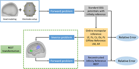
Figure 1. Pipeline for the standard EEG potentials generation, reference transformation, and relative error definition. Given a head model and electrodes setup, the potential with infinity reference is calculated as the ground truth. Later, the standard EEG potentials are transformed to other recordings with different references. Consequently, the relative error between the transformed potentials and the ground truth are cross-compared, regarding reference montages, electrodes setup and some other factors.
Download figure:
Standard image High-resolution imageSpecifically, three-layer head model comprises of brain, skull, and scalp with the conductivities set as 1, 0.0125 and 1, respectively. For the concentric spherical head shape [11, 25], the radii are 1.0, 0.92 and 0.87 for the scalp surface, outer and inner skull surface, separately. The source space consists of 2600 discrete dipoles evenly and radially distributed on the cortical surface with radius r = 0.86 and 1269 * 3 orthogonal dipoles uniformly located in the 3D grid space of subcortical area with radius r ⩽ 0.84. Totally, the accounted dipole number amounts to 6407 for the concentric spherical head model. In addition, the realistic head model is built on basis of the MNI template anatomy ICBM152 [26, 27]. After co-registration with the scalp electrodes, we calculate the forward potentials with boundary element method [28] by OpenMEEG [29] and Brainstorm [30, 31]. Each of the three surfaces (head, inner and outer skull) consists of 1922 vertices with skull thickness set as 4 mm. The source space consists of 15002 * 3 orthogonal dipoles assigned to all the cortical vertices. Thus, 45 006 dipoles in total are considered for the realistic head model.
2.1. Standard EEG potentials generation
With head model and electrode coordinates, the lead field matrix  is calculated with the size of
  (number of channels) by
  (number of dipole sources). Given the activity strengths x of all dipole sources at one moment, the potentials over all electrodes are generated by the equation,

It should be noted that the lead field matrix K is with infinity reference (IR) [32, 33]. Namely, the association between source activities and multichannel potentials is based on a neutral reference at infinity. Here, the EEG generative model is a linear combination of the activities of all dipole sources at each instant. Thus, the EEG potentials are fully determined by the sources at the same instant under the given head model and electrodes setup. Since reference problem is due to the activity of a dipole source arriving at both active electrode and reference site, it is therefore unnecessary to consider the temporal process. We just consider the potentials at one instant in this study. In the following, all the dipole sources are evaluated in turn to minimize the biased effect due to the subjective selection of source positions. Thus, totally  by
by  standard potentials are generated for the error comparison. Certainly, due to the linearity of the equation (1), any combination of different sources can be evaluated similarly.
2.2. Sensor noise test
Realistically, it is inevitable to mix the sensor noise into the recorded EEG signal. We adopt the zero-mean multivariate Gaussian distribution to generate the sensor noise e that may come from various unknown sources. Thus, the EEG generative model (1) changes to
where 0 is a  by 1 zeros vector and
  are a
are a  by
by  identity matrix;
  is the power ratio of the pure EEG signal
  to the sensor noise e in dB unit;
  means the square of the
  norm.
norm.
2.3. Electrodes setup
We investigated 11 channel numbers and two types of electrodes layouts which may affect the accuracy of the EEG potentials. They are 10, 16, 21, 32, 64, 85, 96, 128, 335 channels with '10-x' layout, and 129, 257 channels with 'GSN' layout displayed in figure 2. In detail, about the 3D electrode Cartesian coordinates, 10, 16 and 21 channels are picked from 10-20 system [20]; 32, 64, 96 and 128 channels with '10-10 c' layout are selected from ActiCHamp 128Ch Standard (Brain Products Co. Ltd, Germany); 129 and 257 channels are from the HydroCel™ Geodesic Sensor Net E001 (Electrical Geodesics, Inc., USA); 64 channels with '10-10 n' layout, 85 channels with '10-10 r' layout and 335 channels are from the 10-05 system [18].
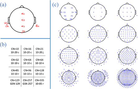
Figure 2. Electrodes setup. (a) shows the five mono-polar reference electrodes, that is, LE, Fz, Pz, Oz, Cz and 2 mastoids (Lm, Rm) used for linked mastoids (LM). The table in (b) summarized the channel number (CN) and electrode layouts where '10-20 c'—clinically used 10-20 system; '10-20 j'—international 10-20 system standardized by [20]; '10-10 c'—commercially available 10-10 system (Brain Products Co. Ltd, Germany); '10-10 n'—standard 10-10 system extended by [21]; '10-10 r' and '10-05 r'—10-10 and 10-05 system defined by [18]; 'GSN 129/257'—Geodesic Sensor Net polygon placement system innovated by [24]. (c) Shows the details of the electrode layouts.
Download figure:
Standard image High-resolution image2.4. Reference montages
In general, all the reference transforming processes can be formulated as

where  is the EEG potentials with infinity reference, T denotes reference transforming matrix that is specific reference dependent,
  is the potentials transformed with a reference notated by
  .
.
2.4.1. Recording references.
The principle of mono-polar recording reference is to subtract the potential at the mono-polar physical reference electrode from each of the active electrodes. Thus,

where 1 is a  by
by  ones vector, and f is a
  by
by  vector with only one non-zero entry (i.e. 1) at the corresponding row of a mono-polar reference, such as LE, Fz, Pz, Oz, and Cz.
2.4.2. Re-references.
Re-reference is a further step based on the measured EEG potentials where the online recording reference process was involved inherently.
Linked mastoids (LM)

where f is the vector with two non-zero entries (i.e. 0.5) at the corresponding rows of left and right mastoids.
Average reference (AR)

where f is with all the entries being  .
.
Reference electrode standardization technique (REST)
Plugging the equations (1) and (4) into (3), we have  . According to the equivalent source principle [11, 25], the scalp potential
  generated by x through lead field K can be generated equivalently by the equivalent sources x1 through lead field
  , i.e.,

Here,  could be the equivalent distributed sources over a 2D cortical sheet that covers the actual sources inside, the 3D distributed sources overlapped with the actual sources, or the multipolar sources at the origin of a coordinate system [25]. For REST, although the true sources x and true lead field K are unknown, we can take the supposed equivalent sources x1 and the related lead field K1 [11, 12]. In this work, 3D grid dipole sources with orthogonal orientation and cortical dipole sources with fixed radial orientation are adopted as x1 for the spherical head model and the realistic head model, respectively.
As the EEG inverse solution is reference independent [34, 35], the approximate estimate of x1 is
By substituting the equations (8) and (3) into (7), the EEG potentials  with infinity reference could be reconstructed as

Therefore, the reference transforming matrix for REST is  .
.
For clarity, all the reference montages are summarized in table 1.


2.5. Head model perturbation test
Essentially, the performance of REST depends on the exactitude of head model, since  is changed from K accordingly with the equivalence between
  and x. Assuming that
  is approximate to K, we are curious about whether REST is sensitive to a perturbation of head model. In previous studies, the perturbation is subjectively added to electrode locations [15] or by means of changing the conductivities [11, 12]. This subjective perturbation is retested over 64 channels ('10-10 c' layout) by recalculating
  as the perturbated
  with various combinations of two head shapes, 11 skull conductivities and five source configurations detailed in section 3.7.
To be more general,  is given an objective perturbation supposed to be together from imprecise estimates of head shape, conductivity, electrode location and other unknown factors that are difficult to concretely quantify in practice. By putting the equations (1) and (9) together, it becomes
Ideally, both  and
and  should be computed by accurate head model and electrode layout. Here,
  is calculated with the accurate head model and true sources, and
  should be calculated with a disturbed head model and assumed equivalent sources. To add perturbation, zero mean multivariate Gaussian noise
  is injected to the lead field vector
  corresponded to the
  dipole source of
  as
as
where  denotes the power of
  to the power of noise ratio in dB unit.
Accordingly, the REST reconstruction model is transformed to
Here, we take the change from  to
to  as the model perturbation.
2.6. Effects evaluation
Given by a head model, the values of lead field are varied with channel number and electrodes layout. By setting the activity of single dipole source with unit strength and the others being zero, the multichannel EEG potentials numerically equal to the lead field vector corresponding to that dipole source. Therefore, the EEG potentials are affected by the electrodes setup. To evaluate the effects, the relative error is taken as a measure for all channels or the partial sensors over one local scalp region. The relative error of the potentials generated by the  dipole is as follows,
where  is the channel number (i.e. array size) or the number of partial sensors over one local scalp region,
  is the forward EEG potentials with one electrodes setup,
  is the EEG potentials with the specific reference. To avoid the bias of source position, we calculate the mean relative error as to numerous dipole sources at the population level rather than a single dipole at the individual level. In the source space or a source region of interest, the relative error (RE) is redefined as
where  is the total number of the dipoles in the source space or one source region. Furthermore, the standard deviation (SD) is calculated as
to evaluate the robustness as to the dipole source position.
3. Results
Comparing the REs before and after reference transforming, we aim to find how the acquired EEG potentials are affected by the factors of interest. In this section, firstly, the REs over all sensors are compared among all the reference montages; afterwards, the effects of channel number and electrodes layout are analyzed; then, compared results of REs are reported as to dipole source position and orientation, as well as sensor noise; lastly, we present the effect of channel number by using realistic head model. Prior to the results, we state that (1) both head models are tested by the identical simulation and analyzing pipeline; (2) since the results for both are quite similar, the figures 3, 4, 6, 7 and 8 are only the results of three-layer concentric spherical head model, while figures 5 and 9 show the comparison of both as to electrodes layout and head model perturbation, respectively.
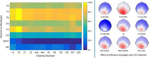
Figure 3. Potential relative error as to reference montages. To differentiate the two 64-channels, '64c' and '64n' hereafter mean 64 channels with '10-10 c' and '10-10 n' layout, respectively. The color in each square corresponds to the RE (in percentage) in the colorbar. The RE is the mean of potential relative errors by repeated simulation with 6407 dipoles individually activated. The standard deviation (SD) of the relative errors over 6407 dipoles are shown in figure 4, especially for AR and REST. Topographies with the same colorbar show the effects (RE in percentage) of all the reference montages compared with infinity reference (IR).
Download figure:
Standard image High-resolution image
Figure 4. Potential relative error as to channel number. The charts separated by the dash lines show the REs of all arrays (10-335), sparse array (⩽32) and dense array (⩾64), respectively. The Y axes are displayed in 10-base logarithm scale. The REs and SDs (error bar) are the mean and standard deviation of the relative error of the potentials over all sensors, or a partial sensors region.
Download figure:
Standard image High-resolution image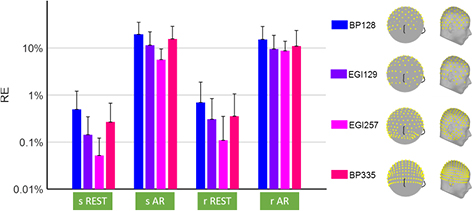
Figure 5. Potential relative error as to electrodes layout. The RE is shown in 10-base logarithm scale, while the prefix 's' and 'r' in the horizontal axis mean the spherical and realistic head model used in simulation, respectively. The legend on the right shows '10-x' layout with 'BP128', 'EGI129' setups and 'GSN' layout with 'EGI257', 'BP335' setups. Each setup is displayed on the spherical and realistic head surfaces with the yellow dots representing the electrode position.
Download figure:
Standard image High-resolution image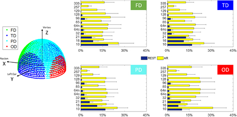
Figure 6. Potential relative error as to dipole source position. The semi-sphere shows the coordinates system and the source space of 3-layer concentric spherical head model. XYZ axes are oriented from the origin to the nasion, towards to the left ear, and directed to the vertex, separately. RE and SD (error bar) are the mean and standard deviation of the potential relative error over all sensors with partial dipoles in one source region individually activated, respectively.
Download figure:
Standard image High-resolution image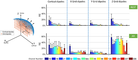
Figure 7. Potential relative error as to source orientation. 3D plot displays the radial orientation of cortical dipoles in blue diamonds and XYZ three orthogonal directions of grid dipoles in red diamonds, respectively. RE and SD (error bar) are the mean and the standard deviation of potential relative error over all sensors with cortical dipoles or grid dipoles individually activated.
Download figure:
Standard image High-resolution image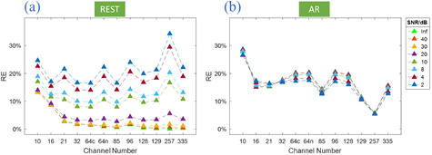
Figure 8. Potential relative error as to sensor noise. RE is the mean of potential relative error over all sensors with all dipole sources individually activated. (a) the effect of REST; (b) the effect of AR.
Download figure:
Standard image High-resolution image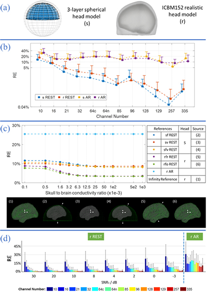
Figure 9. Potential relative error as to head model. (a) The two head models. (b) The REs of potentials generated by the two head models. (c) The effects of perturbated 'r REST' on '64 c' electrodes setup by using different skull conductivities, head shapes, source configuration; the black bar shows 6 source configurations where white arrows display the orientations of dipole source: (1) 17 volume layers and 15 765 * 3 orthogonal dipoles (2) equivalent distributed source layer with 2600 radial cortical dipoles and 400 dipoles perpendicularly to the transverse plane, (3) 1269 * 3 orthogonal volume dipoles, (4) the combination of (2) and (3), (5) 15 002 radial cortical dipoles, and (6) 15 002 * 3 orthogonal cortical dipoles. The prefix of REST in the table, 's, r' means head shape; 'f, v, fv' means 'cortical surface dipoles', 'volume dipoles', and 'surface and volume dipoles', separately; 'r, o' as the third letter denotes radial and orthogonal orientation, respectively. (d) the results of perturbated 'r REST' by injecting noise to the lead field.
Download figure:
Standard image High-resolution image
3.1. Effect of reference montages
The image with scaled colors in figure 3 shows the REs of the potentials over all sensors as to eight reference montages. Without re-reference, the RE is above 61.5% by the mono-polar references (LE, Fz, Pz, Oz, Cz); it reduces to around 41% after re-reference by LM. Especially, the utilization of AR and REST leads to less biased potentials with RE being around 17% and 2.7%, respectively. This means (1) re-reference is indispensable to correct the large biased impacts of mono-polar recording reference; (2) both REST and AR have superiorities to LM; (3) REST is the best among all the reference montages to correct the potentials over all sensors. Eight topographies around the central one with infinity reference (IR) illustrate the effects of reference montages over 257 channels. The central one shows the distribution and strength of standard potentials generated with five cortical dipoles. After reference transforming, the potentials with eight references are plotted in the same colorbar as that with IR for comparison. Apparently, relatively large color change in the topographies referenced by LE, Fz, Pz, Oz, and Cz indicates the distortion effects of online recording reference, while three topographies in the bottom show the correction by offline re-references.
3.2. Effect of channel number
From this section, the comparison will be focused on REST and AR due to their superiorities. The effect of channel number is evaluated in terms of sparse arrays and dense arrays. In addition to all sensors (AS), we calculated the REs over partial sensors as well. Based on the topological conventions, AS is portioned into partial sensors, that is, frontal sensors (FS), temporal sensors (TS), parietal sensors (PS) and occipital sensors (OS). 2D electrodes layout in figure 4 shows how we divided 64 sensors via the red lines. Due to the symmetry between the left TS and the right one, only the RE over the left TS is considered.
Since Y-axes in figure 4 are in 10-base logarithm scale, it is therefore evident that AR has much higher REs than REST over AS and over partial sensors with dense arrays. Over partial sensors with sparse arrays, the REs of REST are still much lower than the REs of AR with 21 and 32 channels; with 10 and 16 channels, the REs of REST are large but still less than the REs of AR. This means that REST enables to outperform AR even with quite sparse arrays. The less REs of REST than AR are found not only over AS but also over partial sensors. These indicate that REST may always correct the EEG potentials with a better performance than AR without the effect of channel number.
The REs of AR do not present the trends of linearly decreasing with increased channel numbers. It implies that dense channels may fail to improve the performance of AR. Namely, channel number or sensor density is not critical to AR. This finding is not in agreement with the general consensus that the advantage of AR only comes into a large number of electrodes and extensive coverage of the head [36]. Lastly, the SDs of REST are always smaller than the SDs of AR. Together to say, REST is more robust than AR in repeated simulations regardless of channel number and scalp region.
3.3. Effect of electrode layout
Much attention should be paid to the dense arrays from 128 to 335 channels, considering the entirely dissimilar electrodes layouts. Figure 5 shows the comparisons of REs between'10-x' layout with 'BP128', 'BP335' setups and 'GSN' layout with 'EGI129', 'EGI257' setups. Each setup is displayed on the spherical and realistic head surfaces to offer an intuitive view of its placement. 'BP128' and 'BP335' are following '10-10 c' and '10-05' systems, with only upper surficial area of the head evenly covered by plenty of electrodes. By contrast, in addition to the different electrodes positioning rule, extensive areas such as the cheek and neck are covered with 'EGI129' and 'EGI257'. REs in figure 5 as to four setups are 0.50%, 0.14%, 0.05%, 0.27% for 's REST' and 19.56%, 11.50%, 5.67%, 15.65% for 's AR', respectively. It is apparent that both REST and AR produce lower RE as to 'GSN' layout compared with '10-x' layout. This shows that the extensive coverage benefits to REST but mainly brings about the great improvements to AR. With almost same channel number but electrodes positions rearranged from 'BP128' to 'EGI129' layout, the RE of AR declines from 19.56% to 11.50%. Whereas, adding 200 more electrodes to 'BP128' and forming into 'BP335' with a quite high spatial sampling and dense coverage, we found that the RE of AR only showed a slight drop from 19.56% to 15.65%. However, the RE of AR with 'EGI257' reduces to be nearly 1/3 of the RE of 'BP335' but with only around 80 (i.e. 335-257) channels removed. Similar results are obtained if the realistic head model (r) is used in place of the three-layer concentric spherical head model (s). These comparisons reveal that on one hand, the key factor to the effect of AR is extensive coverage rather than the large channel number; on the other hand, REST has the appreciably superiority to AR when playing with large number of electrodes.
3.4. Effect of source position
Given electrodes setup and head model, the EEG potential is still affected by the dipole source position. We classify 2600 cortical dipoles and 1269 * 3 orthogonal grid dipoles into four regions based on the conventional division of brain volume. The semi-sphere in figure 6 shows how all dipole sources are divided into fontal dipoles (FD), temporal dipoles (TD), parietal dipoles (PD) and occipital dipoles (OD), individually. The bar plots in figure 6 are with respect to the REs of potentials over all sensors generated by the dipoles located in one source region of interest. The REs generated by FD, TD, PD and OD are shown in the bar plots from top left to bottom right in turn. The REs of REST and AR are shown in blue and yellow bars, respectively. Overall, REST always produces much less REs than AR as to whichever dipole source region.
3.5. Effect of source orientation
In addition to source position, its activated orientation may have serious effects on the accuracy of acquired potentials. Figure 7 shows the REs of the potentials generated by a radial cortical dipole or a grid dipole activated along one of XYZ orthogonal directions, separately. The REs between REST and AR do not manifest such considerable difference in X and Y orientations as that in Z orientation, whereas it shows more prominent similarity between REST and AR in Y orientation than that in X orientation. For the radial cortical dipoles, the extent of RE difference between REST and AR seems to be the compromise of the differences along X, Y and Z orientations. These results may be related to the goodness of symmetry of electrodes position. Close attention is paid back to figure 2 where we see the perfect symmetry between the left and right regions, quite good but imperfect symmetry for the front and back regions, extremely poor symmetry for the top and bottom regions if the 2D electrodes layouts converse to 3D layouts over a spherical or realistic head model shown in figure 5. Additionally, the similar REs as to dipole source orientation reveals that REST is robust to correct the potentials. Much larger REs in radial and Z orientation than X and Y orientations of AR may warn us that AR is subject to dipole source orientation and it is only suitable for dipole sources oriented in the transverse plane.
3.6. Effect of sensor noise
Figure 8 shows the comparison of sensitivity to sensor noise between REST and AR. The case without sensor noise is corresponded to the SNR = Inf dB. From brick red triangles to blue ones, SNRs are 40, 30, 20, 10, 8, 4 and 2 dB, respectively. Markers in the same color are connected to each other to display the waving trends of REs with the change of channel number. It is obvious that the gaps between the dash curves in figure 8(a) are larger than the gaps in figure 8(b). The dash curves in figure 8(a) are lower than the curves in figure 8(b), except for the extensive coverage by 257 channels with SNR < 20 dB and the cases of SNR ⩽ 4 dB where AR reaches a little better effect than REST with some array sizes, such as 21, 64, 96 and 257. These suggest that (1) REST may be of larger sensitivity to sensor noise than AR; (2) REST could be preferred if the EEG is mixed with little noise (3) AR may be acceptable for high noisy situation, due to the possible denoising effects by simply averaging.
3.7. Effect of head model
Figure 9(a) displays three-layer concentric spherical head model (s) and ICBM152 realistic head model (r). We conducted the same simulation and analysis by using 'r' head model as that by using 's' head model. The REs comparison between REST and AR based on the potentials generated by the 'r' and 's' head models are shown in figure 9(b). Big gap between the dash curves in red and purple proves that 'r REST' still enables to obtain quite lower REs than 'r AR' for all the channel numbers. It suggests that the validity of REST may not rely on the complexity of head shape. To check if REST depends on the exactitude of head shape, skull conductivity and source configuration when the truths of these three factors are unknown for someone who underwent the EEG recording, the standard potentials with infinity reference were generated with 'r' head shape, skull to brain conductivity being 0.0125, source configuration as (1) in the black bar of figure 9(c), but the EEG potentials were reconstructed by REST with various combinations of head shape ('s', 'r'), skull to brain conductivity ratio (0.0001, 0.0005, 0.0016, 0.0032, 0.0063, 0.0125, 0.025, 0.05, 0.1, 0.5, 1), and source configuration (2)–(6). Apparently, the superiority of REST over AR can be kept with the simple 's' head shape, skull to brain conductivity being 0.0001, source configuration as the quite different source configurations (2)–(6). It is reasonable to see that the REs of REST decreased with better approximation of head shape, skull to brain conductivity ratio, and source configuration adopted in simulation. To mimic more general situations of the imprecise head model, we tested head model perturbation for 'r REST' by injecting noise. The test results are shown in figure 9(d). Obviously, 'r REST' still enables to have lower REs than 'r AR' even with twice noise (−3dB) injected into the lead field  used for REST. Overall, these results may reveal that REST is insensitive to the perturbation of head model and its advantage can be kept even with the imprecise head model.
4. Discussion
Prior studies have recognized the importance of neutral reference estimation and electrodes layouts to standardize the EEG recordings. For example, acquisition of EEG data by bipolar, unipolar and average reference methods were compared by [37] as early as in 1965; REST was proposed by Yao as the approximate infinity reference [11]; Quanying found that the high-density array was crucial for AR and a realistic head model was critical to REST [15]; 10-20, 10-10 and 10-5 systems were revisited concerning their validity of relative head-surface-based electrodes positioning systems [19]. However, none of them have investigated both multiple optional reference montages and various electrodes setups simultaneously. In this study, we thoroughly investigated the extent to which the measured EEG scalp potentials being affected by reference montage and electrodes setup regarding channel number, scalp region, electrodes layout, dipole source position and orientation, as well as sensor noise and head model.
We found that re-reference should be applied to correct the highly biased EEG potentials with mono-polar recording references and REST could be a better promising reference than the widely adopted AR. For channel number, REST shows much better performances than AR not only for all sensors but also for partial sensors. A surprising outcome is that the effect for AR is not improved with large channel number, whereas the extensive electrode coverage is crucial for AR. This does not follow the statement that the use of AR with dense arrays may still be considered as the 'gold standard' [38, 39]. Additionally, REST enables to produce much lower error than AR wherever dipole sources are located. Moreover, we found that AR may be only suitable for the dipoles oriented in the transverse, while REST is stable under whichever orientation dipole sources are along. Furthermore, REST is a bit more sensitive to the sensor noise but with generally better performance than AR for usual cases. Lastly, repeated analysis with realistic head model and the perturbation test reveal that the advantage of REST can be kept even with the imprecise head model.
These findings may imply that REST is robust to reconstruct the EEG potentials while AR is subject to the electrode coverage and dipole sources orientation. The distinctive differences may be interpreted from the theoretical assumption of AR and REST in physics. For AR, it was assumed that surface integral of potentials over a conductor will be zero [40–42]. New result shows that the integral may not be zero for a realistic head surface [43], thus the zero integral assumption of AR is no longer a general truth even with whole surface sampling being possible. Furthermore, it is impractical to have a balanced coverage such as placing sufficient electrodes on the face, neck, and chin to make the integral being approximate zero as what is required by AR. Namely, the bottom half surface of head is hard to be such densely covered as the scalp. Nevertheless, inhomogeneous tissues and anisotropy conductivity ratio makes it impossible to be zero for the surface integral. The results of AR validate the discussion of Yao [43]. In contrast, REST utilizes the fact that equivalent source could be taken as the intrinsic bridge to link one EEG reference to another. Simply put, although the actual source inversion is nonunique, the EEG potentials with any non-infinity reference can be reconstructed approximately by means of the uniqueness of equivalent source. The easiest way to realize REST is to solve the inverse problem by minimum norm based on the lead field matrix with recording reference and to take the forward calculation again in the Matlab toolbox [44].
This study extends the work of Quanying [15] mainly on utilizing well-established three-layer concentric spherical head model originated in [11] in combination with various reference montages and many more electrodes setups. Our results differ from the findings of Quanying in three aspects, as detailed below: firstly, the crucial factor for AR is if it meets the wide extensive coverage rather than the sensor density; secondly, the superiority of REST exists for all channel numbers and electrodes layouts investigated here; thirdly, although REST is head model dependent, its advantages are not sensitive to the perturbation of head model. To our knowledge, it is the first study to such thoroughly investigate the reference montages and electrodes setup on how to affect the accuracy of EEG recording. These findings may provide helpful suggestions on how to obtain the EEG potentials as accurately as possible for cognitive neuroscientists and clinicians. However, some limitations are worth noting. Although boundary element method is adopted to build the realistic head model, a well-known incorrect assumption is an isotropic conductivity within all regions of each tissue type [45]. Finite element method or finite difference method proposed by [46] offers the possibility to have more accurate conductivity particularly of the skull than boundary element method [47, 48]. Besides, the accuracy of EEG potentials referred here is only in terms of the potential relative error, due to the instantaneous effects of volume conduction. However, spatiotemporal analysis, time-frequency analysis even source imaging may also be affected by the reference montages or electrode layouts [8, 49–55]. Therefore, future studies should be put efforts toward these directions.
5. Conclusion
This study thoroughly investigated the extent to which reference montage and electrodes setup affecting the accuracy of EEG potentials. It is shown that AR and REST are two effective re-references with superiorities to monopolar or linked mastoids references. In view of channel number, scalp regions, electrodes layout, dipole sources position and orientation, as well as sensor noise and head model, it was demonstrated that REST is more robust to correct the distorted potentials than AR, and found that AR is of no relation to sensor density but subject to electrodes coverage and dipole source orientation. We thus recommend the wide attempts of REST and highlight the extensive electrodes coverage to the utilization of AR in the EEG studies.
Acknowledgments
The authors declare no conflict of interest. This research was co-funded by the National Natural Science Foundation of China projects (No. 81571759, 61673090 and 81330032) and the 111 project No. B12027.