
Semi-parametric regression model for survival data: graphical visualization with R
Author’s introduction: Dr. Zhongheng Zhang is a fellow physician working at Sir Run Run Shaw Hospital. He graduated from School of Medicine, Zhejiang University in 2009, receiving Master Degree. His major research interests include hemodynamic monitoring in sepsis and septic shock, delirium, and outcome study for critically ill patients. He is experienced in data management and statistical analysis by using R and STATA, big data exploration, systematic review and meta-analysis. He has published more than 50 academic papers (science citation indexed) that have been cited for over 700 times. He has been appointed as reviewer for 10 journals, including Journal of Cardiovascular Medicine, Hemodialysis International, Journal of Translational Medicine, Critical Care, International Journal of Clinical Practice, Journal of Critical Care.

Abstract: Cox proportional hazards model is a semi-parametric model that leaves its baseline hazard function unspecified. The rationale to use Cox proportional hazards model is that (I) the underlying form of hazard function is stringent and unrealistic, and (II) researchers are only interested in estimation of how the hazard changes with covariate (relative hazard). Cox regression model can be easily fit with coxph() function in survival package. Stratified Cox model may be used for covariate that violates the proportional hazards assumption. The relative importance of covariates in population can be examined with the rankhazard package in R. Hazard ratio curves for continuous covariates can be visualized using smoothHR package. This curve helps to better understand the effects that each continuous covariate has on the outcome. Population attributable fraction is a classic quantity in epidemiology to evaluate the impact of risk factor on the occurrence of event in the population. In survival analysis, the adjusted/unadjusted attributable fraction can be plotted against survival time to obtain attributable fraction function.
Keywords: Survival analysis; nonparametric model; Cox proportional hazards; population attributable fraction; relative hazard
Submitted May 06, 2016. Accepted for publication Jun 20, 2016.
doi: 10.21037/atm.2016.08.61
Introduction
A fully parametric hazard function describes the basic underlying distribution of survival time and how that distribution changes as a function of covariates. If we want to describe the circuit life span in continuous renal replacement therapy as a function of serum ionized calcium and pH value, a fully parametric hazard function is required. However, if we want to see whether circuit life span is longer under acidosis (pH<7.35) when compared with that under normal condition, a complete description of survival time is of secondary importance to a description of how serum pH value modifies the survival time (1). A full description of survival time requires assumption of underlying mathematical model, which may be unnecessarily stringent and unrealistic. Survival time model that leaves its dependence on time unspecified but has a fully parametric regression structure is called semi-parametric regression.
The general form of hazard function is written as:

Where  reflects how hazard function changes with survival time, and
  characterizes how hazard function changes with covariates. Cox has proposed exponential function for r(), and the hazard function is written as:

when x changed from x0 to x1, the hazard ratio is
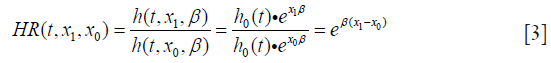
In the literature, the model is termed Cox proportional hazard model (2). Researchers are interested in the parameter β, which is interpreted as changing rate of hazard when the covariate changed by (x1 − x0) unit. Note that the baseline hazard function  remains unknown, that is why the model is called semi-parametric model (3).
Cox proportional hazard model
Ovarian cancer survival data (ovarian) is used to illustrate fitting a Cox proportional hazard model. The study investigated survival in a randomized trial comparing two treatments for ovarian cancer (4).

The fitting Cox regression model appears pretty easy with only one line of R code. The function Surv() creates a survival object. Right side of “~” symbol lists covariates and they are connected with “+” operator. The last argument specifies the dataset containing covariates. Coxph() returns an object of class coxph, containing parameters and statistics we are interested in. the summary() function gives a general glimpse of the content of coxph object. There are 26 observations and 12 of them have the event of interest. The next table shows the coefficients of corresponding covariates. Exponentiation of coefficient gives the hazard ratio. Age is significantly associated with hazard and hazard increases by 1.16 times with each year increase in age. Variable age is denoted by double “*” symbols, suggesting a statistical significance with P<0.01.
The index of concordance (Concordance =0.798 in our example) is a “global” index for validating the predictive ability of a survival model. It is the fraction of pairs in the data, where the observation with the higher survival time has the higher probability of survival predicted by your model. Concordance is equivalent to the area under the ROC curve in logistic regression model. A value of 1 indicates perfect agreement, and a value of 0.5 is an agreement that the model is no better than chance. In other generalized linear models, R-square represents the proportion of variation that can be explained by the model (5). However, the R-square in Cox model also depends on the proportion of censored values. In other words, a perfectly adequate model may have a low R-square due to high large of censored data. Mathematical details of R-square in Cox regression model have been well described (6-10). The likelihood ratio test explores the difference between model with and without covariates. In the example, this statistic follows a Chi-square distribution with 2 degrees of freedom and thus can be used to obtain P value. Score test can be interpreted in a similar way that the model containing variables rx and age is significantly better than null model.
Stratification
The stratified Cox proportional hazard model allows the forms of underlying hazard function to vary across levels of stratification variable. The general form of stratified Cox model is written as:

where j is the number of levels in Z. The covariate Z is adjusted for without estimating its effect. Someone may ask the question: why not incorporate Z as a covariate instead of using it as a stratification factor? The reason is that the predictor may not satisfy proportional hazards assumption and it can be very complex to model hazard ratio for that predictor as a function of time. Furthermore, stratification allows for graphical checks of the proportional hazards assumption. A drawback of stratification is that stratifying unnecessarily (proportional hazard assumption is met) reduces estimation efficacy.

The output of stratified Cox model is similar to the previous one. However, coefficient for age is not estimated because it is now used as stratification factor. Instead, two coefficients are estimated for variable rx, showing that the treatment effects are beneficial for young women and it is harmful for those aged over 60 years. One may wish to graphically examine the fitted model. Survival curves of patients with and without treatment stratified by age are depicted. In the survfit() function, a data frame with the same variable names as those that appear in the coxph formula is specified. The curve(s) produced corresponds to a cohort whose covariates equal to the values in newdata. If a covariate is not specified, the mean of the covariate used in the coxph fit is used. The following example specifies patients with and without treatment (rx=1 and 2).

The output shows survival curves of treated and untreated patients, stratified by age group. The first column is survival time. The last two columns display estimated survival probabilities stratified by treatment group. The result can also be visualized with the following syntax (Figure 1).


Visualization of relative importance of covariates
The interpretation of fitted Cox proportional hazards model depends on regression coefficients, significance level and prevalence of covariate patterns. Also, subject-matter audience may be interested in the importance of covariates in study population. In other words, the importance of a covariate is determined not only by coefficient but also by its distribution in a population. Karvanen and Harrell proposed the relative-hazard plot to visualize relative importance of covariates in proportional hazards model (11). The basic idea is to rank the covariate values and plot relative hazard against ranks. The relative hazard is scaled to the reference hazard. Reference hazard is related to the median of covariates. From this definition, it is obvious that the relative hazard can vary depending on the distribution of covariate values in a population. Rank-hazard plot can be created using rankhazardplot() function. Let’s first install the package and load it onto the workspace. In order to make comparisons of relative importance for all covariates, a full model including all available covariates is built.

The output of function rankhazardplot() shows the Y-axis range. Covariates are scaled to an interval of [0,1]. By default, the minimum, first quartile, median, third quartile and maximum values of each covariate are reported. Figure 2 shows that treatment is the most important determinant of survival at young age, but becomes less important for old age. Similar to the concept of population attributable fraction that the importance of a risk factor is influenced by its prevalence (12), the X-axis of relative-hazard plot displays scaled covariates for the ranking of their relative importance.

Test the proportional hazards assumption
Interpretation and use of Cox proportional hazards model depends on the proportional hazards assumption. Log-hazard function of proportional hazards model takes the form

This function contains log of the baseline hazard function  and linear predictor
  . x and β are highlighted in bold to represent vectors. The proportional hazard assumption dictates the baseline model as a function of time, not of the covariates. Suppose the covariate x has two levels. A plot of log-hazard over time will produce two continuous curve, one for x=0,
  , and the other for x=1,
 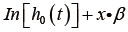 . The difference between the two curves at any time points is β. If log-hazard functions produced by different levels of a given covariate are not equidistant over time, the proportional hazards assumption is violated. Grambsch and Therneau proposed one easily performed test and an associated graph to examine the critical assumption (13).

The cox.zph() function directly performed test for proportional hazards assumption. The output is a table containing rho, Chi-square and P value. Rho is the correlation coefficient between transformed survival time and the scaled Schoenfeld residuals. The correlation coefficient follows a chi-square distribution and the statistic is present in the second column. A P value is given for each covariate. A significant P value indicates that the proportional hazards assumption is violated for that covariate. For the global test there is no correlation and NA is entered into the cell.

Before drawing plots, rows and columns of graphical layout should be specified. The number of panels is determined by the number of covariates. In the example, there are two covariates and thus two panels are defined. If there is only one pannel in the graphical device, only one covariate can be displayed. The Y-axis of the plot is scaled Schoenfeld residuals and X-axis is survival time (Figure 3). The proportional hazards assumption dictates that the residual should not change with survival time. Thus, the smoothed curve should be a flat one. Due to limited number of observations in the example, the sensitivity of the test can be quite low.

Hazard ratio curves for continuous predictors
The Cox proportional hazards model assumes that the continuous predictors are in linear association with log-hazard. However, this assumption may not true in reality. Visualization of the relationship between continuous predictor and hazard ratio helps investigators to check for the linearity assumption. Flexible hazard ratio curve can be plotted using smoothHR package.

The smoothHR() function requires data frame containing covariates and the fitted Cox regression model. The prob argument specifies the reference value of the covariate for hazard ratio. The reference value is the minimum of the hazard ratio curve for prob=0. The hazard ratio curve shows that the age is in linear relation to the log-hazard, but the confidence interval is wide due to small number of observations (Figure 4).

Attributable fraction function
Population attributable fraction (PAF) is defined as
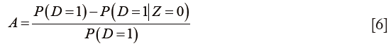
where D is the binary disease status and Z is the binary exposure indicator (14). PAF is defined as “the reduction in incidence that would be achieved if the population had been entirely unexposed, compared with its current (actual) exposure pattern”, and it aims to evaluate the impact of risk factor on the occurrence of event in the population (15). Unlike relative risk, PAF considers the prevalence of risk factors in the population and thus quantifies the population impact of risk factors. PAF can be extended to adjusted attributable fraction (AF) which is defined as the reduction in incidence if some risk factors are eliminated from the population while other risk factors retain their actual levels. When AF is expressed as a function of survival time, it is called attributable fraction function (16). The package paf in R is composed to do the task.
The lung dataset (NCCTG Lung Cancer Data) is employed as worked example (17). Adjusted/unadjusted AF functions of a set of covariates are computed based on the Cox model. The first argument of paf() function is a formula object for the Cox model. Covariates of interest are specified in the cov argument and their AF functions are to be plotted against survival time. In the example, the variable age is investigated for its adjusted and unadjusted (population) attributable fraction function. The solid lines pertain to the point estimates of attributable fraction function and the dashed lines show the 95% confidence limits (Figure 5). It is seen from the figure that after adjustment for covariates the attributable fraction of age is decreased.

Acknowledgements
None.
Footnote
Conflicts of Interest: The author has no conflicts of interest to declare.
References
- Zhang Z, Ni H, Lu B. Variables associated with circuit life span in critically ill patients undergoing continuous renal replacement therapy: a prospective observational study. ASAIO J 2012;58:46-50. [Crossref] [PubMed]
- Cox DR. Regression Models and Life-Tables. Journal of the Royal Statistical Society 1972;34:187-220.
- Hosmer DW Jr, Lemeshow S, May S. Applied survival analysis: regression modeling of time to event data, second edition. Hoboken: Wiley-Interscience; 2008.
- Edmonson JH, Fleming TR, Decker DG, et al. Different chemotherapeutic sensitivities and host factors affecting prognosis in advanced ovarian carcinoma versus minimal residual disease. Cancer Treat Rep 1979;63:241-7. [PubMed]
- Mittlböck M, Schemper M. Explained variation for logistic regression. Stat Med 1996;15:1987-97. [Crossref] [PubMed]
- Kejžar N, Maucort-Boulch D, Stare J. A note on bias of measures of explained variation for survival data. Stat Med 2016;35:877-82. [Crossref] [PubMed]
- Schemper M, Stare J. Explained variation in survival analysis. Stat Med 1996;15:1999-2012. [Crossref] [PubMed]
- O'Quigley J, Xu R, Stare J. Explained randomness in proportional hazards models. Stat Med 2005;24:479-89. [Crossref] [PubMed]
- Xu R, O'Quigley J. A measure of dependence for proportional hazards models. Journal of Nonparametric Statistics 1999;12:83-107. [Crossref]
- Royston P. Explained variation for survival models. Stata Journal 2006;6:83-96.
- Karvanen J, Harrell FE Jr. Visualizing covariates in proportional hazards model. Stat Med 2009;28:1957-66. [Crossref] [PubMed]
- Deubner DC, Tyroler HA, Cassel JC, et al. Attributable risk, population attributable risk, and population attributable fraction of death associated with hypertension in a biracial population. Circulation 1975;52:901-8. [Crossref] [PubMed]
- Grambsch PM, Therneau TM. Proportional hazards tests and diagnostics based on weighted residuals. Biometrika 1994;81:515-26. [Crossref]
- Levin ML. The occurrence of lung cancer in man. Acta Unio Int Contra Cancrum 1953;9:531-41. [PubMed]
- Rothman KJ, Greenland S, Lash TL. Modern Epidemiology. 3rd ed. Philadelphia: LWW; 2012.
- Chen L, Lin DY, Zeng D. Attributable fraction functions for censored event times. Biometrika 2010;97:713-26. [Crossref] [PubMed]
- Loprinzi CL, Laurie JA, Wieand HS, et al. Prospective evaluation of prognostic variables from patient-completed questionnaires. North Central Cancer Treatment Group. J Clin Oncol 1994;12:601-7. [PubMed]

