
The Theoretical and Statistical Ising Model: A Practical Guide in R


1
Department of Psychology, University of Amsterdam, 1105 Amsterdam, The Netherlands
2
Center for Urban Mental Health, University of Amsterdam, 1105 Amsterdam, The Netherlands
*
Author to whom correspondence should be addressed.
Psych 2021, 3(4), 593-617; https://doi.org/10.3390/psych3040039
Submission received: 12 August 2021
/
Revised: 23 September 2021
/
Accepted: 24 September 2021
/
Published: 8 October 2021
(This article belongs to the Special Issue Computational Aspects, Statistical Algorithms and Software in Psychometrics)
Abstract
:The “Ising model” refers to both the statistical and the theoretical use of the same equation. In this article, we introduce both uses and contrast their differences. We accompany the conceptual introduction with a survey of Ising-related software packages in R. Since the model’s different uses are best understood through simulations, we make this process easily accessible with fully reproducible examples. Using simulations, we show how the theoretical Ising model captures local-alignment dynamics. Subsequently, we present it statistically as a likelihood function for estimating empirical network models from binary data. In this process, we give recommendations on when to use traditional frequentist estimators as well as novel Bayesian options.
Keywords:
ising model; alignment; dynamics; binary; networks; computational; estimation; Bayesian; frequentist1. Introduction
The Ising model (named after Ernest Ising. Ironically, Ising concluded that the model was unfit for physics and left science. It was to his surprise that he had become famous through the work of other scientists on the same model [1]) has attracted widespread scientific attention for several decades [1,2,3,4,5,6,7]. Early fascination arose because it was not suspected that such a simple model could produce interesting behaviours. Once its surprisingly complex dynamics were established and used to model magnetic properties, it became one of the most taught and studied models within physics [4,6].
Since its origin in physics, it has spread to several other sciences [5,6,8,9,10,11,12]. Its applications roughly fall into one of two categories. First, it is used as a theoretical model of empirical phenomena. Second, it is used as a data analytic model that provides a statistical likelihood function for dependencies between binary variables. This two-fold use can be explained by its characteristic of being a maximum entropy distribution [12]. From thermodynamics, we know that physical processes maximise entropy [13], which motivates its modeling applications. Additionally, information theory motivates the maximization of entropy given incomplete information [14]. Thus, there is a correspondence between different interpretations of maximum entropy and the Ising model’s applications.
In this paper we focus on its recent use in the expanding literature on network modeling and network psychometrics [15,16]. Here, we see its two-fold use both as a theoretical model of political beliefs, attitudes, and depression [17,18,19], and as a psychometric data analytic tool [7,20,21,22,23].
Both uses have been accompanied by software developments that make these techniques accessible to researchers. However, as of yet there exists no systematic treatise that illustrates the dual use of the Ising model in psychological applications. The current paper aims to fill this gap; in the spirit of "learning by simulating", we show readers how to computationally study both the theoretical and statistical properties of the model. We focus on the freely accessible programming language R, where we survey relevant software packages and illustrate their use [24].
The paper proceeds as follows: In the first part we introduce the Ising model as a theoretical model of alignment. Afterwards we explicate the theoretical model by presenting an overview of software packages and employ these to simulate the dynamics of alignment. We finish the section on its theoretical use by discussing mean-field approximations, encoding and practical application.The fourth part of the paper surveys the statistical use of the Ising model by discussing software related to network psychometrics for binary data. Throughout the sections, text boxes exemplify how the software packages are used. We conclude the paper by discussing the practical differences between the statistical and the theoretical Ising model.
2. The Theoretical Ising Model
In this section, we introduce the Ising model as a theoretical model. Conceptually, we view it as a network governed by the process of local alignment. In the next part of the section, we introduce software relevant to deriving local alignment dynamics and show how we can summarise the dynamics as a cusp catastrophe model. Lastly, we discuss variable encodings and illustrate its extensive applications in climate and opinion research.
2.1. A Conceptual Introduction
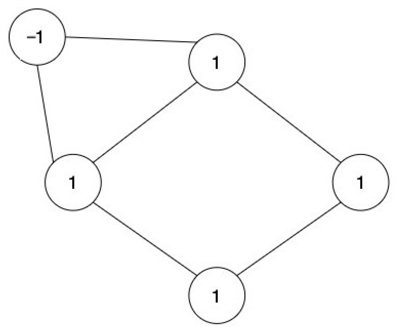
We begin with Figure 1, which shows a general network consisting of five nodes (circle) and six edges (lines connecting the circles). It is general in the sense that nodes and edges can represent any suitable features. As our example, we follow [19], who interprets nodes as attitude elements (such as beliefs, feelings, and behaviours) and edges as their pairwise tendency to align. Following this, we can understand, e.g., a vegetarian attitude as the alignment of meat consumption with beliefs and feelings towards the meat producing industry, climate, health, etc. [19].
If two nodes are connected by an edge, we say they are neighbours. Furthermore, each node i is associated with a variable . More importantly, the Ising model assumes that is dichotomous. Most commonly, is encoded as 1 and −1. For instance, we can code positive-attitude elements with 1 and a negative value with −1. We refer to the value of with . Alternative encodings and their implications are discussed later in this section.
In Figure 1, the current configuration is . This is 1 out of possible configurations. In general, there are possible configurations for n nodes. The Ising model specifies the probability distribution over all network configurations . Where is a vector representing all possible configurations .
2.2. A Model of Alignment
The central assumption of the theoretical Ising model is: the alignment of the current configuration determines how likely it is to occur. Alignment refers to cases where neighbours have the same values (i.e., 1, 1 or −1, −1), whereas divergence happens when neighbours have different values (i.e., −1, 1 or 1, −1). In our simple example, we observe four aligned cases and two that are non-aligned.
The central term of the Ising model is the potential function H, which models alignment as follows (The negative signs in H is the standard notation for the Ising model. It comes from a thermodynamic interpretation where states with the lowest energy/H are the most likely. Note that it is cancelled out by the additional minus sign we see in the exponent of Equation (2)):
where encodes the network structure. If , then i and j are unconnected. If , they are connected with the value of , reflecting the edge strength. Hence, means that we sum up all neighbours (six pairs in our case). Finally, is the external field parameter, which can also be interpreted as an intercept. It gives nodes a directional preference regardless of their neighbours. We see that aligned neighbours and alignment with the external fields make positive contributions to H (assuming all parameters are positive). From the full Ising equation, we see that H drives up the overall probability of the configuration:
The numerator in Equation (2), Z, sums up all configurations, making sure that the probabilities sum up to 1:
This term is called the normalizing constant or the partition function. With more than 20 nodes, Z becomes intractable to calculate due to the computations. Many of the later mathematical tricks that we encounter—sampling methods, expected values, and pseudo-likelihoods—are essentially ways of avoiding the computation of Z.
Equation (2) also contains the parameter, which we refer to as the alignment weight because it weighs the importance of H on . We show this in the next section. The parameter is often referred to as the inverse temperature due to its original ferromagnetic interpretation [1], and sometimes as the density parameter [25].
The Ising model enables us to understand how alignment processes and external influences interact. To do so, we must study which network configurations arise when the external field and alignment weight are varied. We encourage readers to construct their own simulations and insights. In the next section, we will make this process easy and available. To assist us, Table 1 gives an overview of relevant functions in R.
3. Simulating Ising Dynamics
In this section we simulate dynamical processes using an Ising model. This requires two elements: a network structure and the dynamics that determine the progression of the system over time. The network structure is encoded as an adjacency matrix in from Equation (2).
3.1. Network Structures
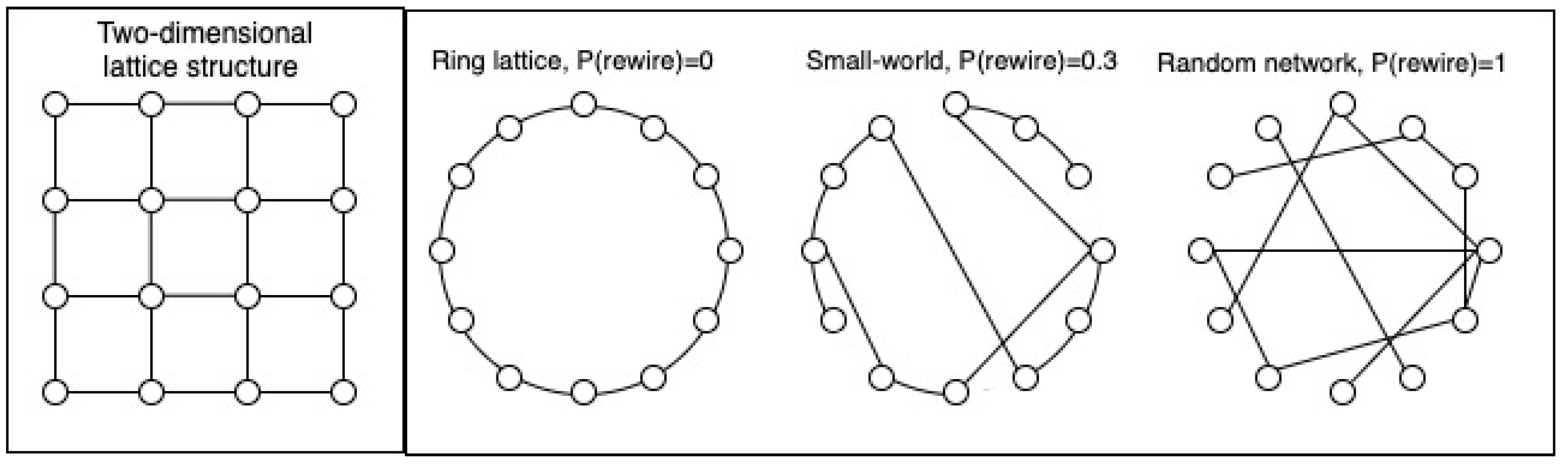
Choosing a network structure is an empirical question that depends on what is being modelled. Ref. [26] discusses commonly found network structures in physics, biology, and social science. Here, we will focus on two simple but general network structures: lattices and the Watts–Strogatz model [27]. Lattices are n-dimensional grid structures (see Figure 2 for a lattice) often used in physics to model atoms. Social and biological networks have been argued to satisfy small-world properties, having both high local clustering and low average distance between nodes. We are not aware of any characteristic structure for psychological networks, although small-world networks have been observed [28,29]. Due to its popularity across disciplines we use it for our simulations. We can obtain small-world networks starting with a ring lattice (see Figure 2) followed by randomly rewiring edges. If this process is continued, we obtain a random graph. Between the ring lattice and random graph, we find the small-world network. It has the local clustering of the ring lattice and low average distances from the random graph. Obtaining small-world properties as a mix of a ring lattice and random graph is referred to as the Watts–Strogatz model. In Text Box 1, we show how lattices and small-world networks are easily generated in R. We also show how to weigh the edges, which is needed to model connections of varying strengths.
Box 1. How to construct common network structures in R [30].

3.2. Equilibrium Configurations
Once we have determined a network structure , we initiate a random configuration. Using Markov chain Monte Carlo algorithms, we can then update the network configurations sequentially such that the system’s time spent in a configuration is equivalent to its Ising probability. This way we create a dynamic Ising system unfolding in time (For a smooth dynamics visualisation of an Ising system with varying see http://bit-player.org/2019/glaubers-dynamics. Unfortunately, R is not suited for similar fast dynamics image updating).
We can use the dynamic system to study the stable states it settles into over time. We refer to these as equilibrium configurations [31,32]. Understanding dynamics means studying the equilibrium configurations as we vary its parameters ( and ). To aid this, we will summarise network configurations through their mean-field: . This is the average value of all nodes. For example, if , all nodes are in state 1, and if , all nodes are . These two values indicate perfectly aligned states. If , on the other hand, nodes are randomly fluctuating. In Text Box 2, we show how to simulate the dynamics of as we vary and .
Box 2. How to sample states from an Ising system [33].

3.3. Dynamics of : A Pitchfork Bifurcation
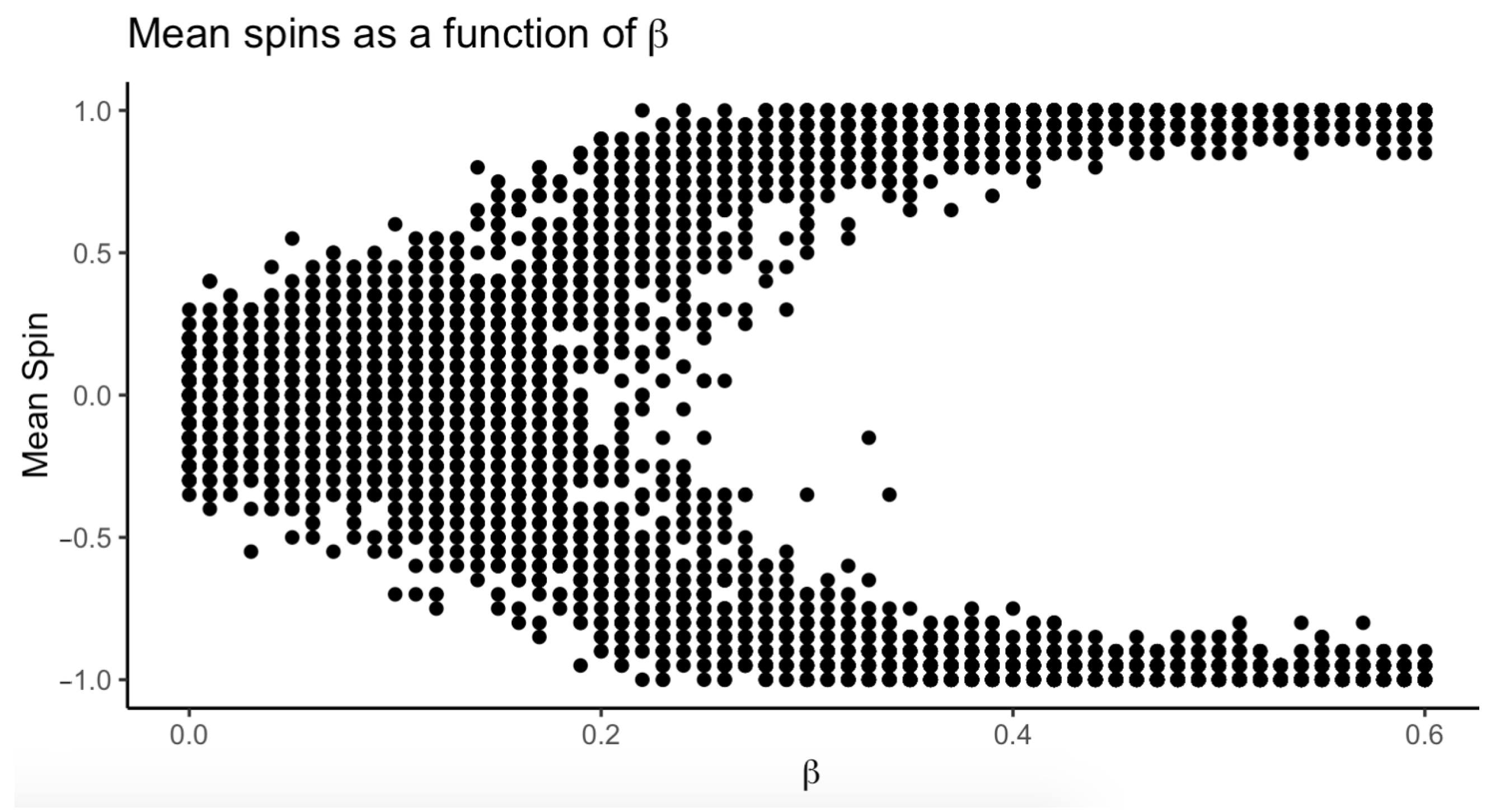
Figure 3 shows the distribution of for different values of (we have assumed ). The resulting pattern is known as a pitchfork bifurcation. A bifurcation refers to qualitative shifts in equilibrium points [31]. The shift happens around . Below this point, the equilibrium is composed of nodes randomly fluctuating, leading to . For , two equilibria diverge towards −1 and 1. Conceptually, the Ising system shifts from a disordered ( to an ordered state () as is increased. The change from disorder to order occurs suddenly at a critical point (this is not very clear from our simulation). This critical point has some remarkable properties that have driven the physical interest in the Ising model [1,2,5]. To our knowledge, disorder to order critical points have not been quantitatively identified for social or psychological phenomena.
Qualitatively, [8] uses the pitchfork bifurcation to model attitude polarisation. This follows from the idea that our attitudes (e.g., towards vegetarianism) are shaped by aligning network elements. Furthermore, if we interpret as involvement, then an increase in involvement leads to more aligned and stronger attitudes. If this process takes place in multiple people with slight initial differences, we expect their attitudes to polarise—following the bifurcation—as involvement increases. Lastly, since amplifies H, it also weighs the importance of if that is a non-zero. If the external field is sufficiently strong relative to the connections, then an increase in leads to nodes being aligned with their respective external fields rather than their neighbours (for further discussion, see [34]).
3.4. Dynamics of : Hysteresis
Otherwise, socio-psychological research tends to focus on the behaviours of the Ising system in the aligned phase—we give multiple examples of this later. Here, the question is about how external influences, , interact with the alignment-driven network. We can easily adapt the code from Text Box 2 to study the dynamics of . Results are presented in Figure 4. More importantly, for this simulation, we assume a high so we are in the alignment-ordered phase. Figure 4 shows that the system has two tipping points, at and [35]. Below and above the tipping points, the system is aligned with the external field. Between the tipping points, the system can be aligned in both directions; as to which one will depend on the history of the system [36]. This dynamic is called hysteresis. We can understand it better by considering our perception of ambiguous stimuli [37].
If we look across the illustrations in Figure 5, we will at some point experience a sudden transition between perceiving a face and a full human posture. Similar to the Ising system, the transition point depends on our starting point. What we perceive between the transition points ambiguously depends on history, similar to the states of our Ising system between and . Furthermore, just after our perception has changed, if we return our gaze to the previous picture, our change in perception is not reversed. Rather, the change in perception persists. To undo the change, we need to go back several figures. This also applies to our Ising system: once we change past one tipping point, we need to turn back to the other tipping point in order to reverse the change. That is the challenge of hysteresis: it is hard to reverse.
3.5. Summarising the Dynamics as a Cusp
So far, we have simulated two cases. We found a pitchfork bifurcation when we varied while keeping . We also found hysteresis as we varied , with . Although this simulation approach is pedagogically useful, it has two shortcomings: (1) It does not give us a mathematical expression relating , , and . (2) It is cumbersome to repeat the simulation for many combinations of and . We can overcome both problems and achieve a relatively simple expression for the dynamics through a mean-field approximation (MFA) [38,39]. In Appendix A, we derive the MFA and perform a graphical bifurcation analysis to derive the dynamics. The central mathematical assumption of the MFA is that nodes interact with a mean field instead of their neighbours. This mean field approximates the effect of the individual interactions between nodes. This is computationally convenient as we avoid computing and Z. The mean field is composed of and the average number of neighbours for the network, . Mathematically, we approximate H as follows (see Appendix A for further explanation):
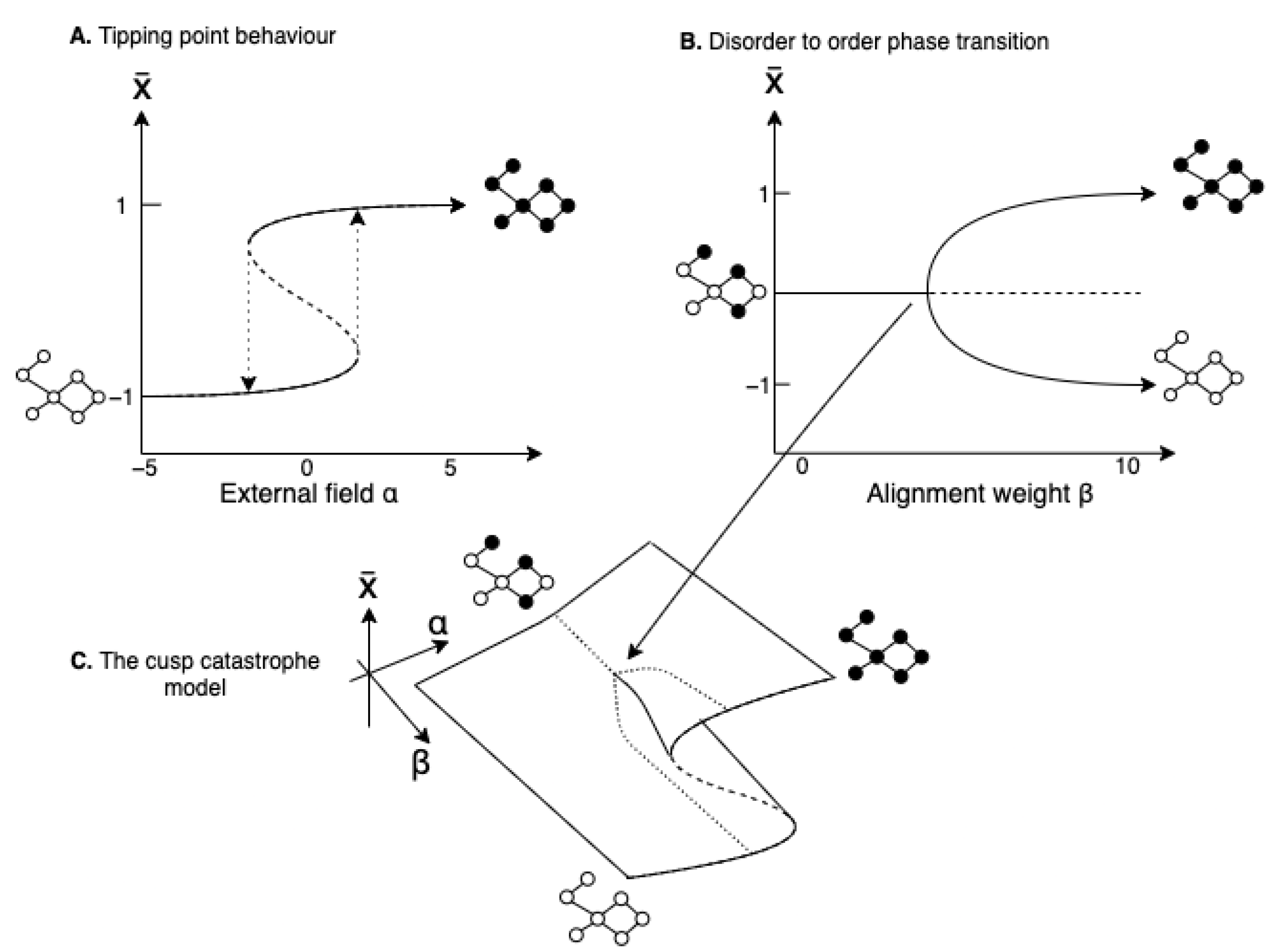
With this simplification and a few extra mathematical steps, we can determine the expected equilibrium points as we systematically vary and . The approximation works better for denser and larger networks [39]. We see the results in Figure 6. Figure 6A shows the hysteresis dynamics arising as we vary while keeping ; Figure 6B shows the pitchfork bifurcation appearing from varying with . Lastly, we can integrate the pitchfork and hysteresis into a single model, as seen in Figure 6C, to get a complete picture of the Ising dynamics. This is the so-called cusp–catastrophe model [31,40].
We can use it to summarise the dynamics of local alignment as follows. The transition from an disordered to an ordered state governed by alignment happens suddenly at a critical point as we increase (pitchfork bifurcation). In the disordered phase, we have linear control over the system’s state through the external field. We lose this control in the alignment’s ordered phase. Here, perturbations of the external field have little impact—the system becomes resilient. That is, until we reach a tipping point after which the entire systems flips. Therefore, alignment induces both resilience but also the capacity for "dramatic" changes [41]. Furthermore, alignment induces two tipping points between which the system’s state depends on its history. This also means that once we pass a tipping point, the change is hard to reverse. The dramatic and hardly reversible changes that are obtained in this region of the model space have inspired the naming of the model as a catastrophe model.
3.6. Variable Encoding
A key assumption of the Ising model is that nodes are dichotomous. However, different encodings are possible. Ref. [42] provides a thorough discussion of this matter, which we will briefly summarise here. There are two generally used options, and . The different encodings make different theoretical assumptions about the dynamics. Nevertheless, we can always transform between different encodings once one is chosen. Ref. [43] covers the mathematical details which are implemented in IsingFit::LinTransform(). We can understand the different consequences of and by considering how they impact the H, and consequently (we leave out, assuming it to be 0):
The alignment of 1 and encoded states decreases H (. This implies an increased probability of the configuration. Thus, configurations with many neighbours aligned at 1 or become likely to occur. We therefore say that the system "wants" to align in both these directions. This is different for variable states coded as . In this case, the alignment of positive states 1 decreases H, but the alignment of 0 does not. In fact, H is unchanged by unaligned and 0 aligned neighbours . Hence, the system does not "want" to align at 0, although it does want to align at 1. This is useful when we model a binary system that only "wants" to align in one direction. Present versus absent symptoms have been modelled this way [18]. In contrast, if the system "wants" to align in either of the directions, then the (−1, 1) encoding provides a better description of the system. Positive versus negative political attitudes have been modelled with this encoding [8,17]. The crucial choice of whether to use the versus configurations depends on whether one theoretically expects negative states to increase alignment; for political attitudes, the hypothesis that negative feelings of a political candidate increase the negative cognitions of that candidate is plausible; meanwhile, for depression, the hypothesis that the absence of one problems causes the absence of another may be less plausible.
3.7. Theoretical Applications
We can regard the theoretical Ising model as a system archetype [44]: a common structure (alignment process in a network) producing a characteristic behaviour (cusp dynamics). Knowledge of system archetypes can help theoretical progress in psychology, a feat many authors have called for [45,46,47,48,49,50]. This is because system archetypes allow researchers to skip the difficult step of crafting a novel model by recognizing that their phenomenon fits an existing one. We see this in a diverse range of fields such as economy [10,51,52], molecular biology [9,53,54], social sciences [11], and biological ecology [55,56,57]. Within psychology, the Ising model has a long-standing tradition of making a good first approximation within opinion research. Both within and across groups of people, opinions are argued to follow alignment processes [17,19,36,58]. More specifically, alignment has repeatedly been linked to our need for consistency of beliefs and aversion towards ambiguity [17,19]. Once this correspondence is established, many hitherto unrelated opinion phenomena can be integrated. For instance, ref. [17] argues that the Ising framework can explain cross-pressures, spillover effects, partisan cues, and ideological differences in attitude consensus. Similarly, ref. [59] argues that an Ising model of attitudes can explain the "mere thoughts" effect, cognitive dissonance, heuristic reasoning, and systematic reasoning. As mentioned, this work is extended by [8] who integrates facts about persuasion to explain political polarisation.
Similar ideas are found in climate research where the notion of tipping points has seen growing attention [60]. Early climate research focused on detecting and preventing environmental tipping points, which can have catastrophic consequences due to their sudden and hardly reversible nature [35,61,62,63]. One strategy of prevention is the enabling of large-scale societal changes. Once again, this has been theorised as possible due to our alignment-driven opinions, which give rise to social tipping points [64,65].
Taken together, these different lines of research converge on the point that opinion dynamics can be approximated by the Ising model. However, we also caution that opinion dynamics are likely to be more complex than any single simple model [66,67]. Therefore, we should regard the Ising model of opinions as a good first approximation while recognising its limitations. Further progress is likely to involve a combination of system archetypes providing a more thorough account of the complexities.
4. The Statistical Ising Model
In this section, we move from the theoretical to the statistical use. We first introduce the statistical application and its software implementations. Table 2 gives an overview of software packages related to statistical Ising estimation. We end this section with some general recommendations for choosing software. Central factors shaping this choice are sample size, network architecture, and further analysis options. We first motivate the recommendations by introducing network psychology, frequentist and Bayesian Ising estimations. As in the previous section, text boxes introduce the software packages in R.
4.1. A Decade of Statistical Ising Models
The Ising model has played an important role for network applications in psychology [15,58,68], where it formed the basis of the estimation of psychometric networks [16,20,69]. Over the last decade, there has been an exponential increase in articles based on network psychometrics [16]. The approach offers an alternative to the standard psychometric view in which psychometric variables are represented as effects of a latent variable [7,70]. Although network psychometrics represents an abstract statistical toolkit that can be used independently of one’s antecedent theory, it aligns naturally with the view that psychological constructs, e.g., depression or conservatism, emerge from networks of causally interacting elements. These elements could be disorder symptoms [15] or our feelings, behaviours, and beliefs [19]. Because we cannot directly observe the interactions between variables, the psychometric challenge is to measure and estimate these. The general solution is to compute the conditional dependence structure from observed data [16,20]. This structure is chosen because it is uniquely identified, in contrast with directed acyclic graphs, and easier to interpret compared to unconditional dependency networks [20]. As we will see, this structure can be estimated from binary data using the Ising model.
4.2. eLASSO Estimation
We can now disregard the alignment interpretations of the Ising model we introduced in the previous section. Instead, we can view the Ising model as a probability distribution that is governed by main effects ( parameters) and pairwise interactions/edges (parameters in ). The model then simply describes the joint probability distribution of a set of variables. We can use it to estimate the so-called pairwise Markov Random Field (pMRF) for binary variables [20,71]. The pMRF represents the probability distribution in terms of pairwise conditional dependencies between variables. Thus, the edges in represent the pairwise dependency after controlling for all other variables (e.g., partial correlations for continuous variables), while absent edges reflect conditional independence [72].
Ref. [69] introduced the estimation of pMRFs using the Ising model to the context of network psychometrics. Similar approaches have been used under various names (homogeneous association model, log-multiplicative association model) in other fields [73,74,75]. Within network psychometrics, ref. [69] developed the elASSO estimator for binary data, which combines pseudo-likelihood estimation with LASSO (Least Absolute Shrinkage Selection Operator) [76]. This combination is now the default estimation process and has since been expanded to ordinal, continuous, and mixtures of variables [23,77].
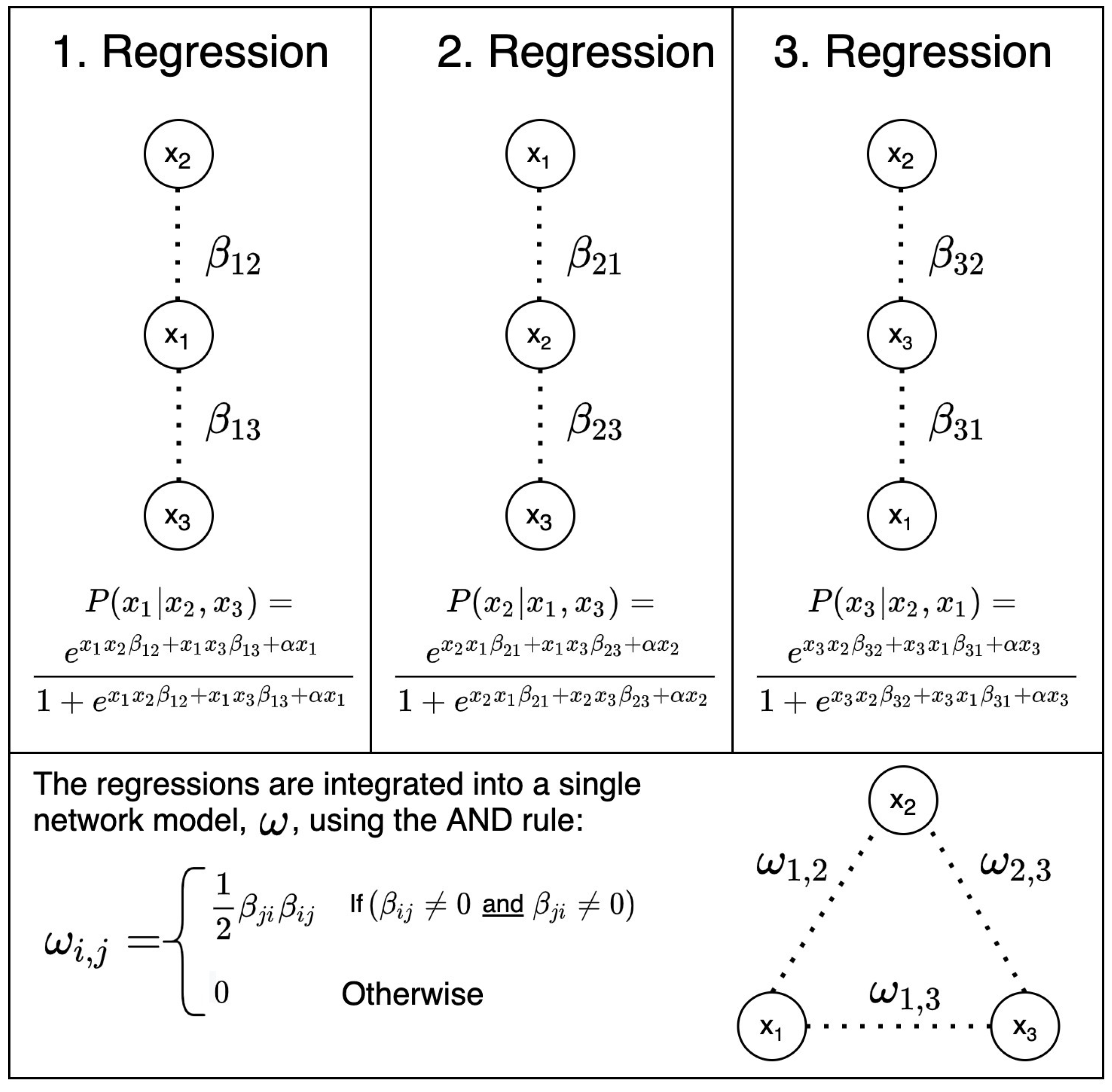
Understanding eLASSO is quite straightforward if one is familiar with logistic regression (see [78] for an introduction). Ref. [69] uses the Ising model as a likelihood function to derive the conditional probability of an observed binary variable given all other measured variables. In Figure 7, this conditional probability is shown for each node of a simple three-node network. More importantly, if , , and are observed variables, this equation translates directly into a logistic regression. Hence, we can estimate and with one regression per node. A caveat is that we will have two estimates per edge, and , because each node serves both as the dependent and independent variables. However, they will converge as sample size goes to infinity. To solve this and complete the adjacency matrix ,69] uses the and-rule: any edge is the average if both and are non-zero, otherwise . A benefit of this node-wise approach is that we avoid computing Z. Consequently, a pseudo-likelihood estimation is needed for large networks.
This multiple logistic regression approach makes it apparent that we are performing multiple testing. This is a central difficulty in hypothesis testing because it inflates the rate of false positives. This issue was recognised by [69] who remedied this problem through LASSO regularisation. This procedure shrinks estimates towards zero, lowering the amount of detected edges and their strengths. The amount of shrinkage depends on a parameter . Choosing the optimal is performed through information criteria-based model selection. This approach to model selection depends on a hyper-parameter . More importantly, this parameter must be set by the analyst as it regulates the error-type control for eLASSO, which means it determines whether false positives or negatives are preferred. Lower favours more edges, while higher favours stronger shrinkage and hence, sparser networks. Therefore, a low increases the false-positive rate, while a high inflates the false-negative rate. We will see that each estimator has a corresponding error-type controller.
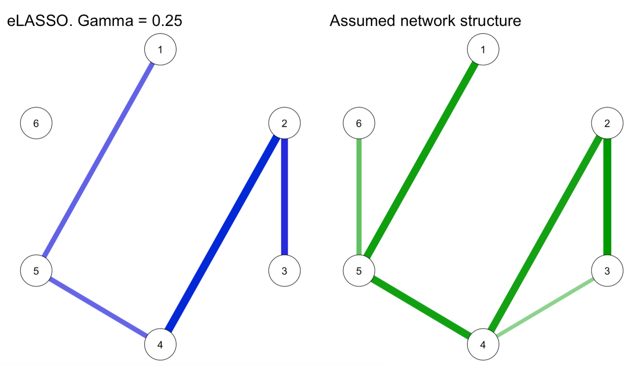
In Text Box 3, we perform eLASSO estimation based on the sample from Text Box 2. We use the default of . The result as well as the original network we generated in Text Box 1 are shown in Figure 8. We see that eLASSO recovers the network well, with two false negatives and no false positives. It should be noted that is usually not identified when we fit statistical Ising models, therefore we do not get an estimate of it. The only exception to this is psychometrics, which allows for its estimation from multi-group data (we will discuss this option later).
The main argument for LASSO is its limiting effect on over-fitting for smaller samples, leading to better out-of-sample generalisability [79]. The sparsity induced by LASSO has also been argued to help to interpret networks as only the most important edges remain [69]. Hence, LASSO is advisable when the goal is to identify important present edges in small to medium samples.
Box 3. How to perform eLASSO estimation with IsingFit.

For larger samples, controlling over-fitting through LASSO becomes less important. Instead, researchers should consider which additional analyses are required (group comparisons, measurement invariance, predictability, missing data handling). In particular, psychometrics and BGGM, which we will cover later, offer extensive additional functionalities.
Besides sample size, the choice of estimator also depends on the theoretical importance of absent edges (or negligibly small effects cf. [80]). Since eLASSO shrinks estimates towards zero, it increases the number of absent edges. The issue for estimated networks is that absent edges arise for two theoretically distinct reasons: (1) the lack of power to detect an existing effect, or (2) the correct detection of zero relation between variables. Since both cases are typically visualised as an absent edge, they are hard to distinguish in practise. This is problematic because they require different conclusions. In the former, we should remain uncertain, while we can build our confidence in no-effects in the latter. Problems arise when they are conflated as we get fooled into building unwarranted confidence in no-effects. Ref. [81] documents several instances of this issue in the literature.
4.3. Bayesian Estimation
We can distinguish the absence of evidence from the evidence of absence with the Bayesian estimation. This is implemented in BDgraph, Rbinnet, and BGGM. Their central difference to eLASSO is their computation of multiple hypotheses per edge . Rbinnet evaluates and . BGGM can perform an expanded three-hypotheses-per-node test: , and . In all cases, we can use to clearly separate the evidence of absence from the absence of evidence.
A central component of Bayesian statistics is prior probabilities allowing researchers to influence the estimation process with background knowledge, as coded in a prior distribution over the parameters of the model. Unless the sample is very large, in which case the prior’s impact becomes negligible, the priors pull estimates towards the center of the prior distribution. Network models involve many parameters, which makes it tricky to set individual prior probabilities. Additionally, little work has been performed on how to set priors for network psychometrics. Here, we suggest one computational workaround. In Text Box 5, we show how to easily compute a robustness analysis. That is, we repeat the analysis with different analysis choices (e.g., priors) to see if the results are robust in these changes.
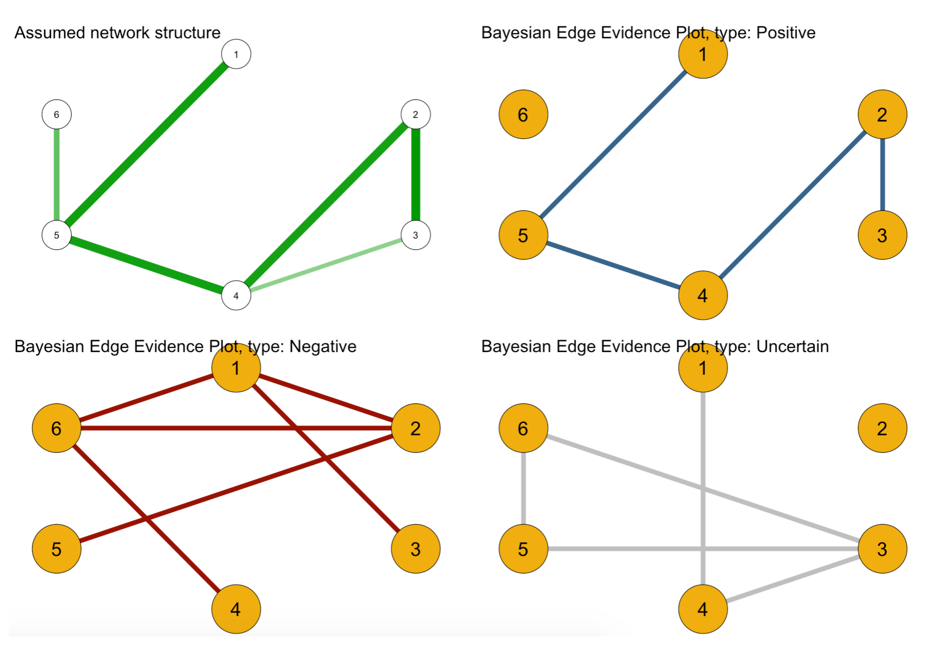
We first perform Bayesian estimation with rbinnet, which is followed by a robustness analysis of the result [82]. We use rbinnet to compute two hypotheses per edge, and . As explained in Text Box 4, we can use the hypotheses to generate a novel edge-uncertainty graph (introduced in [83]). The estimation depends on a prior-inclusion and precision parameter, which we must specify. In Text Box 5, we examine the robustness of the results on changes in the prior-inclusion and precision parameters.
Box 4. How to perform Bayesian Ising estimation using rbinnet. We show this information in three edge-uncertainty graphs in Figure 9.

Figure 9.
Result of rbinnet used to construct edge uncertainty plots. The edges of coloured graphs represent the inclusion Bayes factor . The red graph indicates the evidence of absence of an edge (). The blue graph provides the evidence of inclusion of an edge (). The grey graph shows the absence of evidence ().

Box 5. Robustness analysis of rbinnet results. We see the results in Figure 10.

Figure 10.
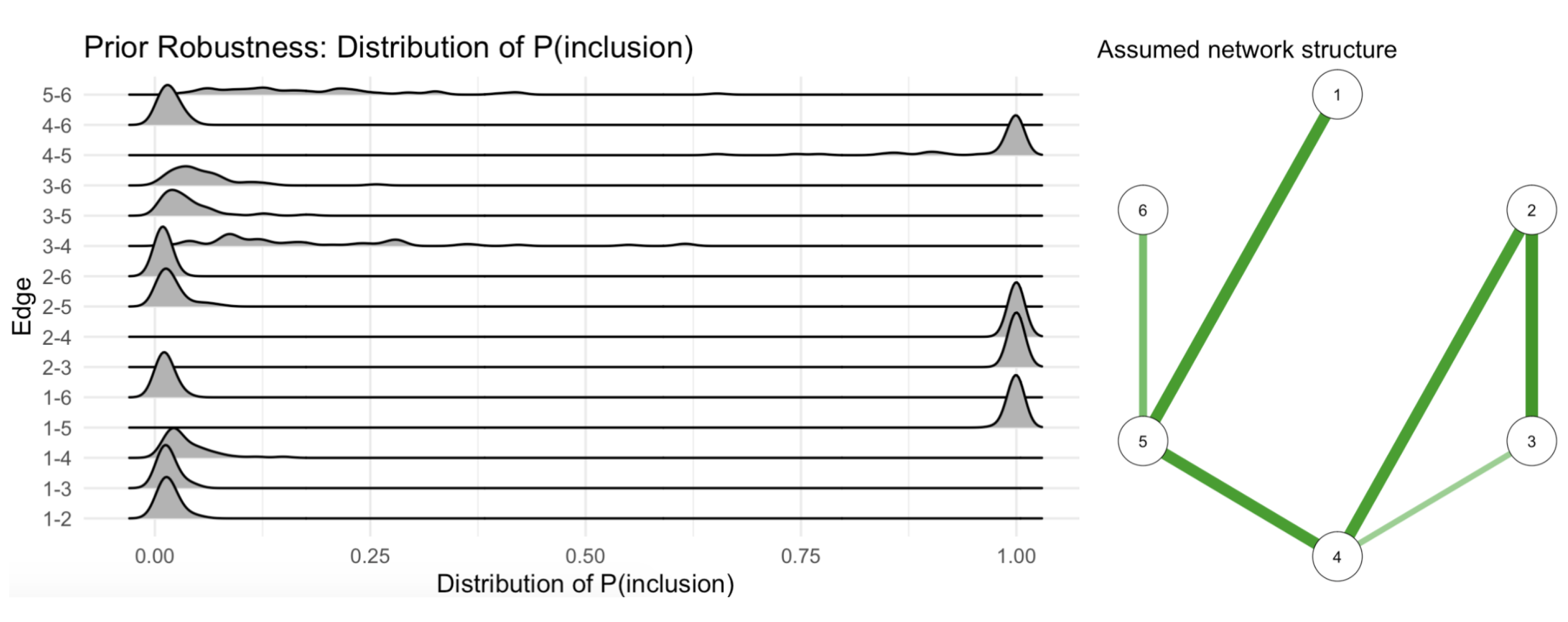
Robustness analysis based on rbinnet. The robustness of posterior inclusion probabilities is studied for various combinations of prior inclusion probabilities and precisions. We see that four edges have consistently high posterior inclusion probabilities (robust)—which are also the strongest in the assumed structure. Two edges have their probabilities “smeared out”, indicating non-robustness. Finally, nine edges have robustly low posterior inclusion probabilities.
Figure 10.
Robustness analysis based on rbinnet. The robustness of posterior inclusion probabilities is studied for various combinations of prior inclusion probabilities and precisions. We see that four edges have consistently high posterior inclusion probabilities (robust)—which are also the strongest in the assumed structure. Two edges have their probabilities “smeared out”, indicating non-robustness. Finally, nine edges have robustly low posterior inclusion probabilities.

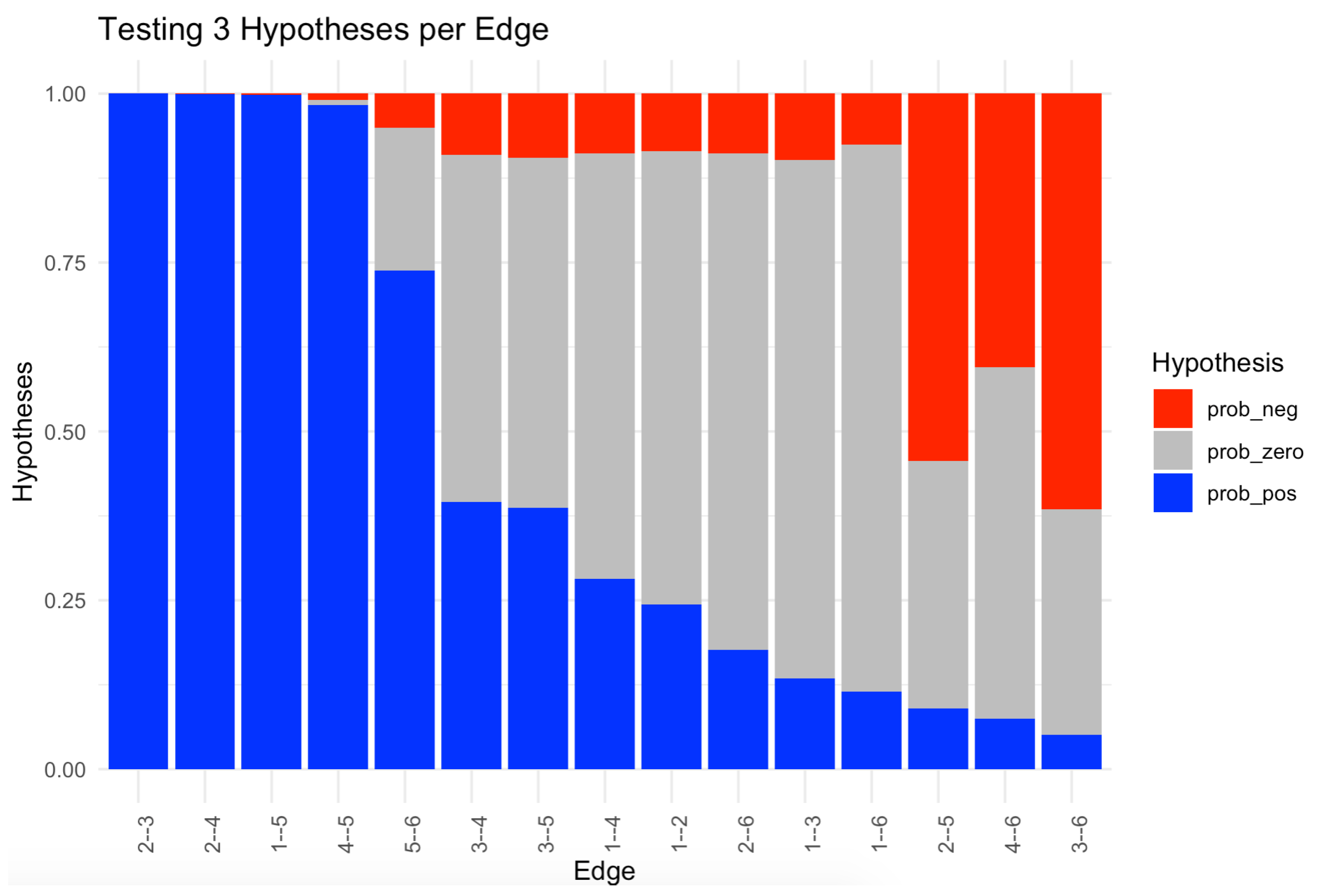
The second Bayesian option is the BGGM (we refer to the general R-package, not the specific estimation procedure of [84]). This package allows not only for exploratory estimation, as we have covered so far, but also for the confirmatory analysis of a pre-specified structure. It is a flexible function that accepts continuous, ordinal, binary, and a mixture of variable types. BGGM also offers a range of extra analysis options; for instance, missing data handling, group comparisons, and node predictability. In Text Box 6, we use BGGM to perform exhaustive hypothesis testing. That is, we test three hypotheses per edge: , , and . As explained in the text box, we used the three hypotheses to create the stacked bar plot of Figure 11.
Box 6. Bayesian Ising estimation using BGGM.

4.4. Maximum Likelihood Estimation
Lastly, it is also possible to estimate Ising models using the maximum likelihood estimation (MLE) with psychometrics. This is a frequentist estimator without LASSO. In Text Box 7, we demonstrate this and explain the pruned MLE estimation. This offers a versatile package that bridges statistical network modelling with structural equation modelling (SEM) [85]. Following SEM, psychometrics allows for model-constraining, which is useful for group comparisons and measurement invariance testing, among others. A noteworthy feature of Ising models is that we can identify through constraints. This requires multiple group data where we then constrain the network structure and external fields in order to be equal. We illustrate how this is executed in the analysis script. In Text Box 7, we estimate a fully saturated and pruned model and compare their fit using psychometrics::compare().
4.5. Summary of Recommendation
In this section, we have covered the use of the Ising model as a likelihood function for parameter estimation. As we have seen, several R packages have implemented Ising estimation methods. The choice of Ising estimator depends on the research question and data. The central question is if further analysis is needed (missing data handling or group comparisons, for instance). In particular, psychometrics and BGGM offer extensive analysis options. Secondly, we highlighted that sample size and interpretability of absent edges are important to estimator choice. eLASSO is well-established and easy to use in small to medium sample sizes where present edges are in focus. For larger samples, full maximum likelihood is preferred over eLASSO. If absent edges are of theoretical importance, Bayesian estimators are good options as they compute the evidence of absence directly.
Box 7. Pruned maximum likelihood estimation using psychometrics. The comparison results are
shown in Table 3.


Table 3.
Output of model comparison using psychometrics. We estimated a saturated model (DF = 0) and a pruned model (DF = 39) from data generated in Text Box 2. A comparison of the two models’ fit indices (AIC and BIC) shows that the pruned model is preferred as it has both lower AIC and BIC.
Table 3.
Output of model comparison using psychometrics. We estimated a saturated model (DF = 0) and a pruned model (DF = 39) from data generated in Text Box 2. A comparison of the two models’ fit indices (AIC and BIC) shows that the pruned model is preferred as it has both lower AIC and BIC.
| Model | DF | BIC | AIC |
|---|---|---|---|
| Model 1: saturated | 0 | 4965 | 4862 |
| Model 2: Pruned | 11 | 4909 | 4858 |
5. The Practical Gap between Statistical and Theoretical Ising Use
In the paper, we have discussed both the statistical and theoretical uses of the Ising model. Although mathematically identical, they will often be used separately. This is because the statistical Ising model provides little evidence for the theoretical one. The theoretical model assumes that the system is alignment-driven based on which we can derive the cusp dynamics. To verify the theoretical model, we should ideally study a system over time in order to observe alignment and its consequent bifurcation and hysteresis behaviour. Subsequently, the statistical model can play an important role in parameter estimation. But the statistical model alone does not provide strong evidence for the theoretical model. This is because of the statistical equivalence between the network, latent variable, and item response-models [7]. The central tenet of the statistical model is that it makes weak assumptions, and consequently yields weak evidence for any specific data-generating structure such as the theoretical Ising model. This is also its strength. This means that it is a suitable tool whenever we want to explore our data and we have little intuition about the data-generating mechanism. In these cases, we can avoid additional theoretical assumptions—unlike latent variable models, directed acyclic graphs, etc.—by estimating the pRMF, which is always uniquely identified. This makes the statistical Ising model a powerful exploratory tool: it identifies a correct data pattern regardless of what the underlying data-generating mechanism is. This result can then inspire and constrain further hypotheses that typically need more substantive information through experimental manipulations or time-series data.
Author Contributions
Conceptualization, A.F., D.B., S.E. and H.L.J.v.d.M.; methodology, A.F.; software, A.F.; validation, D.B., S.E. and H.L.J.v.d.M.; formal analysis, A.F.; writing—original draft preparation, A.F.; writing—review and editing, A.F., D.B., S.E. and H.L.J.v.d.M.; supervision, D.B., S.E. and H.L.J.v.d.M. All authors have read and agreed to the published version of the manuscript.
Funding
This research was funded by Denny Borsboom’s NWO Vici Grant No. 181.029, and Sacha Epskamp’s NWO Veni Grant No. 016-195-26.
Institutional Review Board Statement
Not applicable.
Informed Consent Statement
Not applicable.
Data Availability Statement
All data is simulated using the code found on our OSF.
Acknowledgments
We thank Karoline Huth for her help with using rbinnet and visualising its results.
Conflicts of Interest
The authors declare no conflict of interest.
Abbreviations
The following abbreviations are used in this manuscript:
| MFA | Mean-field approximation |
| MLE | Maximum likelihood estimation |
Appendix A
Here, we briefly derive the mean-field approximation (MFA) of the Ising model (The derivation is inspired by Simon Dedeo’s course on renormalization: www.complexityexplorer.org/courses/67-introduction-to-renormalization/). It consists of two parts. We first derive the MFA expression, which we subsequently perform a bifurcation analysis of in order to determine its expected equilibrium points.
To derive the MFA, we re-write H as the sum of "alignment" for each node i (we assume to be 0, and we omit the double negative sign of the exponent):
The central assumption of the MFA is that nodes interact with an approximation of their neighbours. This approximation is the mean-field, , multiplied by the average number of neighbours in the system, . We approximate the neighbour interaction term as follows:
Conceptually we replace our fine grained description of the system by aggregating the nodes into a single mean field. In this process, we throw out information about individual variation. For a discussion of the MFA’s validity under various network structures, see [39].
We can now inset our re-written H into the Ising equation:
The final step is to eliminate Z. We can accomplish this by obtaining the expected value of a node. We start by finding the probability that a single node is positive:
Each factor gives the probability of its corresponding node being positive. We see that this probability is equal for all nodes:
Based on this, we can obtain the expected value of the node . This is the sum over each possible state value multiplied by its respective probability. Since each node has two states, 1 and −1, we obtain:
We eliminate by using . This leads us to an expression where cancels out in the end:
Lastly, we use a trigonometric rule to rewrite the expression in terms of . This gives us the final mean-field approximation where we also re-inset :
We can think of the MFA as a difference equation that predicts at the next time point given the current mean spin: . The goal is then to find the equilibrium points. They are the values of such that it is equal to , i.e., the output is not changed from the input. A bifurcation analysis amounts to determining these equilibria as we vary and [31]. We take a graphical approach where we plot together with the diagonal . The diagonal is useful because it generally shows where . Therefore, we can find the equilibria of by seeing where it intersects with the diagonal. Figure A1 shows in blue for different values of , assuming . For low values of , we see one intersection so that one equilibrium at . As increases, three equilibriums arise around 1, 0, and . It is important to notice that 0 is an unstable equilibrium, so we do not expect the system to be in this state (see [31] for an explanation). To construct a bifurcation plot, we systematically plot the equilibria as a function of . By doing so, we obtain Figure A2 showing the pitchfork bifurcation we simulated earlier (see Figure 3). Following the same method but varying , we can obtain the hysteresis plot of Figure 6A. Lastly, we trust [31] in that we can integrate our bifurcation analyses into the cusp catastrophe model.
Figure A1.
Equilibrium plots for tanh() with varying .

Figure A2.
The bifurcation plot resulting from plotting equilibrium points of the MFA while varying the alignment weight .
Figure A2.
The bifurcation plot resulting from plotting equilibrium points of the MFA while varying the alignment weight .

References
- Brush, S.G. History of the Lenz-Ising model. Rev. Mod. Phys. 1967, 39, 883. [Google Scholar] [CrossRef]
- Ernest, I. Ising: Beitrag zur theorie des ferromagnetismus. Z. Für Phys. 1926, 31, 253–258. [Google Scholar]
- Onsager, L. Crystal Statistics. I. A Two-Dimensional Model with an Order-Disorder Transition. Phys. Rev. 1944, 65, 117–149. [Google Scholar] [CrossRef]
- Bhattacharjee, S.M.; Khare, A. Fifty years of the exact solution of the two-dimensional Ising model by Onsager. Curr. Sci. 1995, 69, 816–821. [Google Scholar]
- Sole, R.V. Phase Transitions; Primers in Complex Systems; OCLC: Ocn757257299; Princeton University Press: Princeton, NJ, USA, 2011. [Google Scholar]
- Galam, S. Sociophysics: A review of Galam models. Int. J. Mod. Phys. C 2008, 19, 409–440. [Google Scholar] [CrossRef]
- Kruis, J.; Maris, G. Three representations of the Ising model. Sci. Rep. 2016, 6, 1–11. [Google Scholar] [CrossRef] [PubMed] [Green Version]
- van der Maas, H.L.J.; Dalege, J.; Waldorp, L. The polarization within and across individuals: The hierarchical Ising opinion model. J. Complex Netw. 2020, 8, cnaa010. [Google Scholar] [CrossRef]
- Duke, T.A.J.; Bray, D. Heightened sensitivity of a lattice of membrane receptors. Proc. Natl. Acad. Sci. USA 1999, 96, 10104–10108. [Google Scholar] [CrossRef] [Green Version]
- Bornholdt, S.; Wagner, F. Stability of money: Phase transitions in an Ising economy. Phys. A Stat. Mech. Appl. 2002, 316, 453–468. [Google Scholar] [CrossRef] [Green Version]
- Stauffer, D. Social applications of two-dimensional Ising models. Am. J. Phys. 2008, 76, 470–473. [Google Scholar] [CrossRef] [Green Version]
- Roudi, Y. Statistical physics of pairwise probability models. Front. Comput. Neurosci. 2009, 3, 22. [Google Scholar] [CrossRef] [Green Version]
- Martyushev, L.M.; Seleznev, V.D. Maximum entropy production principle in physics, chemistry and biology. Phys. Rep. 2006, 426, 1–45. [Google Scholar] [CrossRef]
- Jaynes, E.T. On the rationale of maximum-entropy methods. Proc. IEEE 1982, 70, 939–952. [Google Scholar] [CrossRef]
- Borsboom, D.; Cramer, A.O. Network analysis: An integrative approach to the structure of psychopathology. Annu. Rev. Clin. Psychol. 2013, 9, 91–121. [Google Scholar] [CrossRef] [Green Version]
- Robinaugh, D.J.; Hoekstra, R.H.A.; Toner, E.R.; Borsboom, D. The network approach to psychopathology: A review of the literature 2008–2018 and an agenda for future research. Psychol. Med. 2020, 50, 353–366. [Google Scholar] [CrossRef] [PubMed]
- Brandt, M.J.; Sleegers, W.W. Evaluating belief system networks as a theory of political belief system dynamics. Personal. Soc. Psychol. Rev. 2021, 25, 159–185. [Google Scholar] [CrossRef]
- Cramer, A.O.J.; van Borkulo, C.D.; Giltay, E.J.; van der Maas, H.L.J.; Kendler, K.S.; Scheffer, M.; Borsboom, D. Major Depression as a Complex Dynamic System. PLoS ONE 2016, 11, e0167490. [Google Scholar] [CrossRef]
- Dalege, J.; Borsboom, D.; Harreveld, F.V.; Lunansky, G.; Maas, H.L.J.v.d. The Attitudinal Entropy (AE) Framework: Clarifications, Extensions, and Future Directions. Psychol. Inq. 2018, 29, 218–228. [Google Scholar] [CrossRef]
- Epskamp, S.; Maris, G.K.J.; Waldorp, L.J.; Borsboom, D. The Wiley Handbook of Psychometric Testing: A Multidisciplinary Reference on Survey, Scale and Test Development; Wiley: Hoboken, NJ, USA, 2016; pp. 953–986. [Google Scholar]
- Fried, E.I.; Bockting, C.; Arjadi, R.; Borsboom, D.; Amshoff, M.; Cramer, A.O.; Epskamp, S.; Tuerlinckx, F.; Carr, D.; Stroebe, M. From loss to loneliness: The relationship between bereavement and depressive symptoms. J. Abnorm. Psychol. 2015, 124, 256. [Google Scholar] [CrossRef] [PubMed] [Green Version]
- Boschloo, L.; Borkulo, C.D.v.; Borsboom, D.; Schoevers, R.A. A Prospective Study on How Symptoms in a Network Predict the Onset of Depression. Psychother. Psychosom. 2016, 85, 183–184. [Google Scholar] [CrossRef] [PubMed]
- Epskamp, S.; Borsboom, D.; Fried, E.I. Estimating psychological networks and their accuracy: A tutorial paper. Behav. Res. Methods 2018, 50, 195–212. [Google Scholar] [CrossRef] [Green Version]
- R Core Team. R: A Language and Environment for Statistical Computing; R Foundation for Statistical Computing: Vienna, Austria, 2020. [Google Scholar]
- Newman, M.; Watts, D. Renormalization group analysis of the small-world network model. Phys. Lett. A 1999, 263, 341–346. [Google Scholar] [CrossRef] [Green Version]
- Broido, A.D.; Clauset, A. Scale-free networks are rare. Nat. Commun. 2019, 10, 1–10. [Google Scholar] [CrossRef] [PubMed]
- Watts, D.J.; Strogatz, S.H. Collective dynamics of ‘small-world’ networks. Nature 1998, 393, 440–442. [Google Scholar] [CrossRef] [PubMed]
- Dalege, J.; Borsboom, D.; Van Harreveld, F.; Van den Berg, H.; Conner, M.; Van der Maas, H.L. Toward a formalized account of attitudes: The Causal Attitude Network (CAN) model. Psychol. Rev. 2016, 123, 2. [Google Scholar] [CrossRef]
- Borsboom, D.; Cramer, A.O.; Schmittmann, V.D.; Epskamp, S.; Waldorp, L.J. The small world of psychopathology. PLoS ONE 2011, 6, e27407. [Google Scholar] [CrossRef] [Green Version]
- Csardi, G.; Nepusz, T. The igraph software package for complex network research. InterJournal 2006, 1695, 1–9. [Google Scholar]
- Strogatz, S.H. Nonlinear Dynamics and Chaos; Taylor & Francis Inc.: Abingdon, UK, 2014. [Google Scholar]
- Guastello, S.J.; Koopmans, M.; Pincus, D. Chaos and Complexity in Psychology; Cambridge University Press: Cambridge, UK, 2010. [Google Scholar]
- Epskamp, S. parSim: Parallel Simulation Studies. Available online: cran.r-project.org/web/packages/parSim/parSim.pdf (accessed on 29 September 2021).
- Dalege, J.; van der Maas, H.L.J. Accurate by Being Noisy: A Formal Network Model of Implicit Measures of Attitudes. Soc. Cogn. 2020, 38, s26–s41. [Google Scholar] [CrossRef]
- Scheffer, M.; Carpenter, S.; Foley, J.A.; Folke, C.; Walker, B. Catastrophic shifts in ecosystems. Nature 2001, 413, 591–596. [Google Scholar] [CrossRef]
- Galam, S.; Gefen (Feigenblat), Y.; Shapir, Y. Sociophysics: A new approach of sociological collective behaviour. I. mean-behaviour description of a strike. J. Math. Sociol. 1982, 9, 1–13. [Google Scholar] [CrossRef]
- Ditzinger, T.; Haken, H. Oscillations in the perception of ambiguous patterns a model based on synergetics. Biol. Cybern. 1989, 61, 279–287. [Google Scholar] [CrossRef]
- Bianconi, G. Mean field solution of the Ising model on a Barabási–Albert network. Phys. Lett. A 2002, 303, 166–168. [Google Scholar] [CrossRef] [Green Version]
- Waldorp, L.; Kossakowski, J. Mean field dynamics of stochastic cellular automata for random and small-world graphs. J. Math. Psychol. 2020, 97, 102380. [Google Scholar] [CrossRef]
- van der Maas, H.L.J.; Kolstein, R.; van der Pligt, J. Sudden Transitions in Attitudes. Sociol. Methods Res. 2003, 32, 125–152. [Google Scholar] [CrossRef]
- Siegenfeld, A.F.; Bar-Yam, Y. An Introduction to Complex Systems Science and its Applications. arXiv 2019, arXiv:1912.05088. [Google Scholar]
- Haslbeck, J.M.; Epskamp, S.; Marsman, M.; Waldorp, L.J. Interpreting the Ising model: The input matters. Multivar. Behav. Res. 2020, 56, 303–313. [Google Scholar] [CrossRef] [PubMed] [Green Version]
- Kruis, J. Transformations of mixed spin-class Ising systems. arXiv 2020, arXiv:2006.13581. [Google Scholar]
- Meadows, D.H.; Meadows, D.L.; Randers, J.; Behrens, W.W. The Limits to Growth; Yale University Press: New Haven, CT, USA, 1972. [Google Scholar]
- Oberauer, K.; Lewandowsky, S. Addressing the theory crisis in psychology. Psychon. Bull. Rev. 2019, 26, 1596–1618. [Google Scholar] [CrossRef]
- Fried, E.I. Lack of theory building and testing impedes progress in the factor and network literature. PsyArXiv 2020. [Google Scholar] [CrossRef] [Green Version]
- Mischel, W. The Toothbrush Problem; Association for Psychological Science: Washington, DC, USA, 2008; Volume 21. [Google Scholar]
- Borsboom, D.; van der Maas, H.; Dalege, J.; Kievit, R.; Haig, B. Theory Construction Methodology: A practical framework for theory formation in psychology. PsyArXiv 2020. [Google Scholar] [CrossRef] [Green Version]
- Robinaugh, D.; Haslbeck, J.M.B.; Waldorp, L.; Kossakowski, J.J.; Fried, E.I.; Millner, A.; McNally, R.J.; van Nes, E.H.; Scheffer, M.; Kendler, K.S.; et al. Advancing the Network Theory of Mental Disorders: A Computational Model of Panic Disorder. PsyArXiv 2019. [Google Scholar] [CrossRef]
- Muthukrishna, M.; Henrich, J. A problem in theory. Nat. Hum. Behav. 2019, 3, 221–229. [Google Scholar] [CrossRef] [PubMed] [Green Version]
- Zhou, W.X.; Sornette, D. Self-organizing Ising model of financial markets. Eur. Phys. J. B 2007, 55, 175–181. [Google Scholar] [CrossRef]
- Hosseiny, A.; Bahrami, M.; Palestrini, A.; Gallegati, M. Metastable Features of Economic Networks and Responses to Exogenous Shocks. PLoS ONE 2016, 11, e0160363. [Google Scholar] [CrossRef]
- Weber, M.; Buceta, J. The cellular Ising model: A framework for phase transitions in multicellular environments. J. R. Soc. Interface 2016, 13, 20151092. [Google Scholar] [CrossRef]
- Matsuda, H. The Ising model for population biology. Prog. Theor. Phys. 1981, 66, 1078–1080. [Google Scholar] [CrossRef] [Green Version]
- Nareddy, V.R.; Machta, J.; Abbott, K.C.; Esmaeili, S.; Hastings, A. Dynamical Ising model of spatially coupled ecological oscillators. J. R. Soc. Interface 2020, 17, 20200571. [Google Scholar] [CrossRef] [PubMed]
- Wang, Y.; Badea, T.; Nathans, J. Order from disorder: Self-organization in mammalian hair patterning. Proc. Natl. Acad. Sci. USA 2006, 103, 19800–19805. [Google Scholar] [CrossRef] [PubMed] [Green Version]
- Bialek, W.; Cavagna, A.; Giardina, I.; Mora, T.; Silvestri, E.; Viale, M.; Walczak, A.M. Statistical mechanics for natural flocks of birds. Proc. Natl. Acad. Sci. USA 2012, 109, 4786–4791. [Google Scholar] [CrossRef] [Green Version]
- Maas, H.L.J.V.D.; Dolan, C.V.; Grasman, R.P.P.P.; Wicherts, J.M.; Huizenga, H.M.; Raijmakers, M.E.J. A dynamical model of general intelligence: The positive manifold of intelligence by mutualism. Psychol. Rev. 2006, 113, 842–861. [Google Scholar] [CrossRef]
- Dalege, J.; Borsboom, D.; van Harreveld, F.; van der Maas, H.L. The Attitudinal Entropy (AE) Framework as a general theory of individual attitudes. Psychol. Inq. 2018, 29, 175–193. [Google Scholar] [CrossRef] [Green Version]
- Milkoreit, M.; Hodbod, J.; Baggio, J.; Benessaiah, K.; Calderón-Contreras, R.; Donges, J.F.; Mathias, J.D.; Rocha, J.C.; Schoon, M.; Werners, S.E. Defining tipping points for social-ecological systems scholarship—an interdisciplinary literature review. Environ. Res. Lett. 2018, 13, 033005. [Google Scholar] [CrossRef]
- Scheffer, M.; Bascompte, J.; Brock, W.A.; Brovkin, V.; Carpenter, S.R.; Dakos, V.; Held, H.; van Nes, E.H.; Rietkerk, M.; Sugihara, G. Early-warning signals for critical transitions. Nature 2009, 461, 53–59. [Google Scholar] [CrossRef] [PubMed]
- Lenton, T.M.; Rockström, J.; Gaffney, O.; Rahmstorf, S.; Richardson, K.; Steffen, W.; Schellnhuber, H.J. Climate tipping points—Too risky to bet against. Nature 2019, 575, 592–595. [Google Scholar] [CrossRef]
- Lenton, T.M. Early warning of climate tipping points. Nat. Clim. Chang. 2011, 1, 201–209. [Google Scholar] [CrossRef]
- Otto, I.M.; Donges, J.F.; Cremades, R.; Bhowmik, A.; Hewitt, R.J.; Lucht, W.; Rockström, J.; Allerberger, F.; McCaffrey, M.; Doe, S.S. Social tipping dynamics for stabilizing Earth’s climate by 2050. Proc. Natl. Acad. Sci. USA 2020, 117, 2354–2365. [Google Scholar] [CrossRef] [PubMed] [Green Version]
- Bentley, R.A.; Maddison, E.J.; Ranner, P.H.; Bissell, J.; Caiado, C.; Bhatanacharoen, P.; Clark, T.; Botha, M.; Akinbami, F.; Hollow, M. Social tipping points and Earth systems dynamics. Front. Environ. Sci. 2014, 2, 35. [Google Scholar] [CrossRef] [Green Version]
- Galesic, M.; Olsson, H.; Dalege, J.; van der Does, T.; Stein, D.L. Integrating social and cognitive aspects of belief dynamics: Towards a unifying framework. J. R. Soc. Interface 2021, 18, 20200857. [Google Scholar] [CrossRef]
- Page, S.E. The Model Thinker: What You Need to Know to Make Data Work for You, 1st ed.; OCLC: on1028523969; Basic Books: New York, NY, USA, 2018. [Google Scholar]
- Borsboom, D. A network theory of mental disorders. World Psychiatry 2017, 16, 5–13. [Google Scholar] [CrossRef] [Green Version]
- Van Borkulo, C.D.; Borsboom, D.; Epskamp, S.; Blanken, T.F.; Boschloo, L.; Schoevers, R.A.; Waldorp, L.J. A new method for constructing networks from binary data. Sci. Rep. 2014, 4, 1–10. [Google Scholar] [CrossRef] [Green Version]
- Fried, E.I. Theories and Models: What They Are, What They Are for, and What They Are About. Psychol. Inq. 2020, 31, 336–344. [Google Scholar] [CrossRef]
- Kindermann, R.; Snell, J.L. Markov Random Fields and Their Applications; OCLC: 1030357447; American Mathematical Society: Providence, RI, USA, 2012. [Google Scholar]
- Cox, D.R.; Wermuth, N. Linear dependencies represented by chain graphs. Stat. Sci. 1993, 8, 204–218. [Google Scholar] [CrossRef]
- Anderson, C.J.; Vermunt, J.K. Log-Multiplicative Association Models as Latent Variable Models for Nominal and/or Ordinal Data. Sociol. Methodol. 2000, 30, 81–121. [Google Scholar] [CrossRef] [Green Version]
- Wickens, T.D. Multiway Contingency Tables Analysis for the Social Sciences; Psychology Press: East Sussex, UK, 2014. [Google Scholar]
- Marsman, M.; Borsboom, D.; Kruis, J.; Epskamp, S.; van Bork, R.; Waldorp, L.J.; Maas, H.L.J.v.d.; Maris, G. An Introduction to Network Psychometrics: Relating Ising Network Models to Item Response Theory Models. Multivar. Behav. Res. 2018, 53, 15–35. [Google Scholar] [CrossRef]
- Ravikumar, P.; Wainwright, M.J.; Lafferty, J.D. High-dimensional Ising model selection using ι1-regularized logistic regression. Ann. Stat. 2010, 38, 1287–1319. [Google Scholar] [CrossRef] [Green Version]
- Haslbeck, J.M.B.; Waldorp, L.J. mgm: Estimating Time-Varying Mixed Graphical Models in High-Dimensional Data. arXiv 2020, arXiv:1510.06871. [Google Scholar] [CrossRef]
- Hosmer, D.W., Jr.; Lemeshow, S.; Sturdivant, R.X. Applied Logistic Regression; John Wiley & Sons: Hoboken, NJ, USA, 2013; Volume 398. [Google Scholar]
- Epskamp, S.; Kruis, J.; Marsman, M. Estimating psychopathological networks: Be careful what you wish for. PLoS ONE 2017, 12, e0179891. [Google Scholar] [CrossRef]
- Meehl, P.E. Why Summaries of Research on Psychological Theories are Often Uninterpretable. Psychol. Rep. 1990, 66, 195–244. [Google Scholar] [CrossRef]
- Williams, D.R.; Briganti, G.; Linkowski, P.; Mulder, J. On Accepting the Null Hypothesis of Conditional Independence in Partial Correlation Networks: A Bayesian Analysis. PsyArXiv 2021. Available online: psyarxiv.com/7uhx8 (accessed on 27 July 2021).
- Marsman, M.; Huth, K.; Waldorp, L.; Ntzoufras, I. Objective Bayesian Edge Screening and Structure Selection for Networks of Binary Variables. PsyArXiv 2020, 26. Available online: psyarxiv.com/dg8yx/ (accessed on 15 July 2021).
- Huth, K.; Luigjes, J.; Goudriaan, A.; van Holst, R. Modeling Alcohol Use Disorder as a Set of Interconnected Symptoms-Assessing Differences between Clinical and Population Samples and Across External Factors. PsyArXiv 2021. Available online: psyarxiv.com/93t2f/ (accessed on 25 June 2021).
- Williams, D.R.; Mulder, J. Bayesian hypothesis testing for Gaussian graphical models: Conditional independence and order constraints. J. Math. Psychol. 2020, 99, 102441. [Google Scholar] [CrossRef]
- Epskamp, S.; Isvoranu, A.M.; Cheung, M. Meta-analytic Gaussian Network Aggregation. PsyArXiv 2020. [Google Scholar] [CrossRef] [Green Version]
Figure 1.
A simple network with five nodes and six edges. Its current configuration is .

Figure 2.
On the left, a two-dimensional lattice structure. On the right, a small-world and a random network are created from a ring lattice by varying the rewiring probability of edges.
Figure 2.
On the left, a two-dimensional lattice structure. On the right, a small-world and a random network are created from a ring lattice by varying the rewiring probability of edges.

Figure 3.
Result of sampling from an Ising distribution, with and varying between 0.00 and 0.06. The simulation assumes the small-world network structure of 40 variables from Text Box 1. Deviations from become more likely for smaller networks and the pitchfork shape less pronounced.
Figure 3.
Result of sampling from an Ising distribution, with and varying between 0.00 and 0.06. The simulation assumes the small-world network structure of 40 variables from Text Box 1. Deviations from become more likely for smaller networks and the pitchfork shape less pronounced.

Figure 4.
Result of sampling from an Ising distribution with (ordered phase) and varying between −6 and 6. The simulation assumes the small-world network structure of 40 variables from Text Box 1. We see the outline of a hysteresis effect.
Figure 4.
Result of sampling from an Ising distribution with (ordered phase) and varying between −6 and 6. The simulation assumes the small-world network structure of 40 variables from Text Box 1. We see the outline of a hysteresis effect.

Figure 5.
A series of ambiguous stimuli used by [37] to illustrate hysteresis. By looking across the illustrations in the figure, one will experience a transition in perception. This transition point depends on the direction we started from. Figures that are in between the transition points are ambiguous.

Figure 6.
The cusp catastrophe model (C) presents a unified picture of the alignment dynamics arising from the dynamical Ising model. It encompasses pitchfork bifurcation (B) and hysteresis (A).
Figure 6.
The cusp catastrophe model (C) presents a unified picture of the alignment dynamics arising from the dynamical Ising model. It encompasses pitchfork bifurcation (B) and hysteresis (A).

Figure 7.
With a pseudo-likelihood estimation, we first estimate the neighbourhood of each node. This is performed through one logistic regression per node (here, we consider a simple three-node example). The bottom panel shows how we combine the neighbourhoods into a single network model, , through the AND rule: an edge is present if both and are non-zero. This step is necessary because each node is both the dependent and independent variables; hence, we have two estimates.

Figure 8.
To the right, the "true" network structure (Text Box 1), which we simulated at 1000 observations per node from Text Box 2. To the left, we estimated the network using .

Figure 11.
With , we compute three hypotheses per edge: (grey), (blue), and (red). The absence of evidence then amounts to equal probabilities across the edge hypotheses.
Figure 11.
With , we compute three hypotheses per edge: (grey), (blue), and (red). The absence of evidence then amounts to equal probabilities across the edge hypotheses.

Table 1.
Software packages in R relevant in the simulation of Ising Dynamics. We relate functions to their packages using the ‘::’ notation from R. To access a function, we first install its package with install.package(“Example”) then load the package with library(“Example”).
Table 1.
Software packages in R relevant in the simulation of Ising Dynamics. We relate functions to their packages using the ‘::’ notation from R. To access a function, we first install its package with install.package(“Example”) then load the package with library(“Example”).
| Package::Function() | Description |
|---|---|
| IsingSampler::Isingsampler() | Flexible Ising state sampler |
| bayess:isinghm() | Metropolis–Hastings Sampler |
| igraph::make_lattice() | N dimensional lattice structures |
| igraph::sample_small_world() | Watts–Strogatz model |
| parSim::parSim() | Easy simulations and multi-core |
| ggplot2::ggplot() | Visualisation |
| set.seed() | Reproduces random numbers |
Table 2.
Software packages in R relevant to estimating Ising models from binary data.
| Package::Function() | Description | Pros | Cons | Encoding |
|---|---|---|---|---|
| IsingFit::IsingFit() | eLASSO estimation | Small–medium samples detecting present edges Applicable to >20 variables | Large samples Interpreting absent edges | (1, 0) |
| psychometrics::Ising() | Full maximum likelihood | Large samples Extensive further analysis options | Small samples Max of 20 variables | Any |
| mgm::mgm() | eLASSO | For mixtures of binary, continuous, and ordinal variables | Large samples Interpreting absent edges | (1, 0) |
| rIsing::Ising() | eLASSO | Small–medium samples Detecting present edges Applicable to >20 variables | Large samples Interpreting absent edges | (1, 0) |
| rbinnet::select_structure() | Bayesian estimation Slap and spike prior | Evidence of absent edges Model uncertainty Prior information use | Work in progress Prior information dependent | (1, 0) |
| BGGM::explore(type = “binary”) | Bayesian estimation F-matrix prior | Evidence of absent edges Model uncertainty Prior information use | Prior information dependent | (1, 0) |
| BDgraph::bdgraph() | Bayesian model selection G-wishart Prior | Model uncertainty Prior information use | Prior information dependent | (1, 0) |
| IsingFit::LinTransform() | Transforms between (1, 0) and (1, −1) encodings | Works with unregularised models (psychometrics) | Any | |
| NetworkComparisonTest::NCT() | Group comparison test | Works with eLASSO models |
Publisher’s Note: MDPI stays neutral with regard to jurisdictional claims in published maps and institutional affiliations. |
© 2021 by the authors. Licensee MDPI, Basel, Switzerland. This article is an open access article distributed under the terms and conditions of the Creative Commons Attribution (CC BY) license (https://creativecommons.org/licenses/by/4.0/).
Share and Cite
MDPI and ACS Style
Finnemann, A.; Borsboom, D.; Epskamp, S.; van der Maas, H.L.J. The Theoretical and Statistical Ising Model: A Practical Guide in R. Psych 2021, 3, 593-617. https://doi.org/10.3390/psych3040039
AMA Style
Finnemann A, Borsboom D, Epskamp S, van der Maas HLJ. The Theoretical and Statistical Ising Model: A Practical Guide in R. Psych. 2021; 3(4):593-617. https://doi.org/10.3390/psych3040039
Chicago/Turabian StyleFinnemann, Adam, Denny Borsboom, Sacha Epskamp, and Han L. J. van der Maas. 2021. "The Theoretical and Statistical Ising Model: A Practical Guide in R" Psych 3, no. 4: 593-617. https://doi.org/10.3390/psych3040039