Deep-ACTINet: End-to-End Deep Learning Architecture for Automatic Sleep-Wake Detection Using Wrist Actigraphy

Abstract

Sleep scoring is the first step for diagnosing sleep disorders. A variety of chronic diseases related to sleep disorders could be identified using sleep-state estimation. This paper presents an end-to-end deep learning architecture using wrist actigraphy, called Deep-ACTINet, for automatic sleep-wake detection using only noise canceled raw activity signals recorded during sleep and without a feature engineering method. As a benchmark test, the proposed Deep-ACTINet is compared with two conventional fixed model based sleep-wake scoring algorithms and four feature engineering based machine learning algorithms. The datasets were recorded from 10 subjects using three-axis accelerometer wristband sensors for eight hours in bed. The sleep recordings were analyzed using Deep-ACTINet and conventional approaches, and the suggested end-to-end deep learning model gained the highest accuracy of 89.65%, recall of 92.99%, and precision of 92.09% on average. These values were approximately 4.74% and 4.05% higher than those for the traditional model based and feature based machine learning algorithms, respectively. In addition, the neuron outputs of Deep-ACTINet contained the most significant information for separating the asleep and awake states, which was demonstrated by their high correlations with conventional significant features. Deep-ACTINet was designed to be a general model and thus has the potential to replace current actigraphy algorithms equipped in wristband wearable devices.

1. Introduction

Quality of sleep is crucial for physical and mental health and thus could affect human lives, socially and financially [1,2]. There is indeed a variety of sleep disorders, such as sleep related breathing disorders, hypersomnia, parasomnia, circadian rhythm disorders, and sleep related epilepsy [3], that have been affecting the daily activities of human beings [4,5]. Sleep stage estimation, or so-called sleep scoring, therefore plays an important role in improving human lives, by helping to diagnose sleep disorders and evaluate the quality of sleep.

Polysomnography (PSG), which has been used for adaptive segmentation to classify sleep stages [6] and for the detection of sleep disorders using multi-modal bio-signals and movement information from video polysomnography [7,8], is one of these sleep monitoring methods. Because PSG is complex, expensive, and uncomfortable for subjects, another simple method, actigraphy, which scores sleep stages based on movement detection from a wristband device, has also been utilized [9]. This method enables subjects to perform the experiments in their familiar and comfortable home environments [10]. In addition, sleep monitoring based on the pressure-body movement-sleeping model [11] has been conducted, employing a flexible force sensitive sensor mattress to gather and monitor pressure signals from the subject.

Traditionally, sleep scoring analysis of actigraphs has been achieved via preprocessing, statistical feature extraction, and linear classification algorithms based on activity based sleep-wake identification [12]. Among the various traditional methods, the Cole–Kripke [13] and Sadeh [12] algorithms, which could distinguish between sleeping and awake states using predefined rule based models, are the most popular. However, these methods are quite vulnerable to unexpected deviations of input data patterns, caused by ambient noises or movement artifacts, owing to their handcrafted methods [14,15].

Conventionally, machine learning methods have been applied for physical abnormality detection [16,17]. Especially, sleep scoring using machine learning has shown great success. Dhongade et al. utilized linear discriminant analysis (LDA) and principle component analysis (PCA) to extract features from electroencephalogram (EEG) signals and then classified them into either sleep disorder or normal [18]. Moeynoi and Kitjaidure conducted sleep stage scoring using statistical features of EEG signals via simple statistical techniques and canonical correlation analysis to obtain the correlations among the feature vectors of the dataset [19]. For sleep scoring application, five machine learning methods, which include the kstar classifier, bagging, random committee, random subspace, and random forest, were applied by Yeo et al. [9] in a study where features of accelerometer data from a wristband sensor were trained and classified into wake, rapid eye movement (REM), and light and deep stages. The naive Bayes algorithm, which has been utilized to predict sleep apnea severity and sleepiness [20], was trained based on demographics and polysomnogram and electrocardiogram EEG signals. However, several conventional machine learning algorithms depend on feature engineering, which is based mostly on predefined and handcrafted models and thus could be suboptimal for nonstationary and nonlinear biosignal data [21].

Recently, deep neural networks (DNNs) have been developed and have remarkably improved classification performances in various areas of study [22]. A DNN model using convolutional neural network (CNN) has been applied to the classification problem of sleep scoring based on EEG data [23,24] and electrocardiogram (ECG) data [25]. CNN has been, moreover, employed for activity recognition based on wrist worn accelerometer data [26], where CNN outperformed conventional machine learning algorithms such as SVM and LDA. In [27], a sequential CNN model outperformed the other CNN structures like multi-task learning based CNN. The CNN architecture has an advantage of capturing high level information that is directly related to the problem [28]. However, researchers still are using predefined model based features [29], such as Fourier based synchronization features using handcrafted sinusoidal basis functions [30], before the CNN classification process.

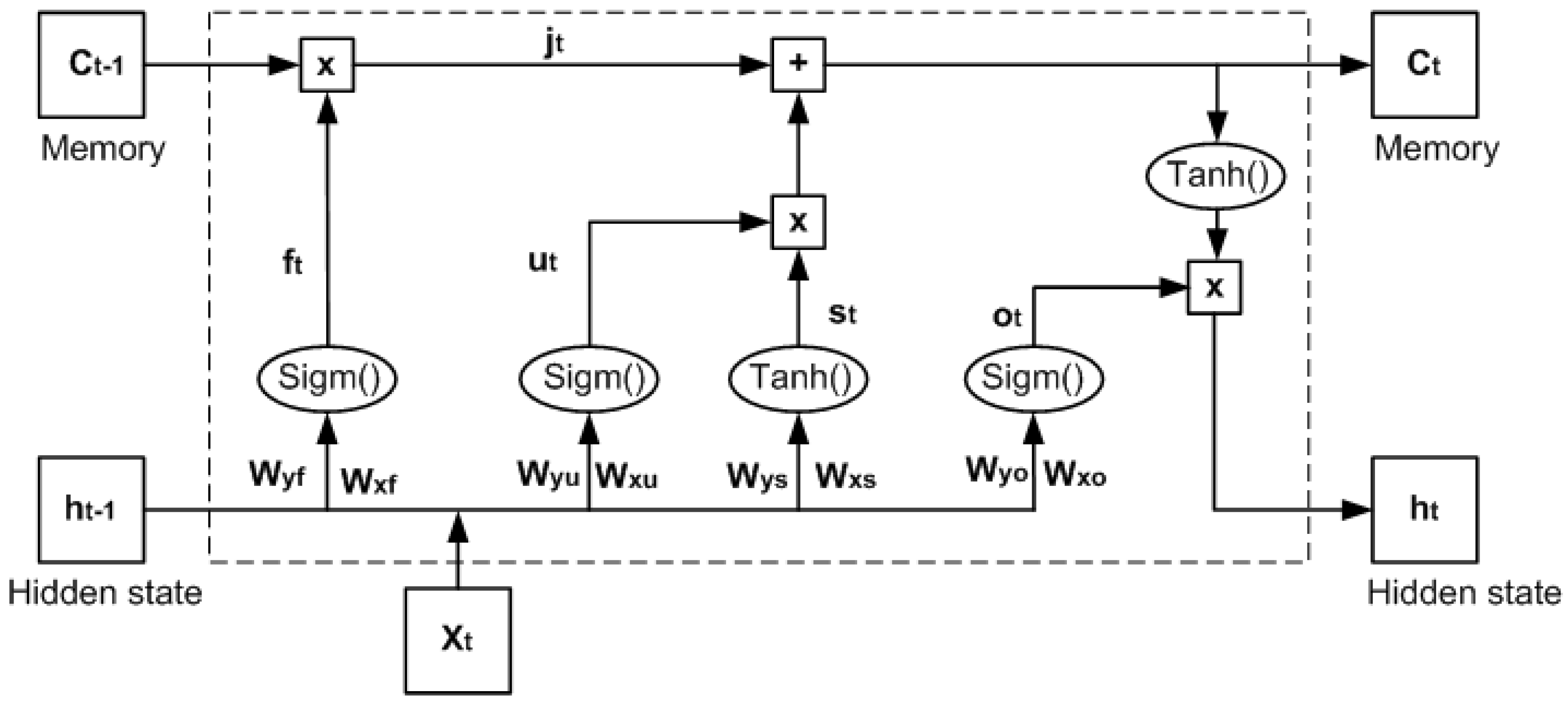
For sleep analysis, long short term memory (LSTM) has also been studied extensively. LSTM was used for the temporal sleep scoring based on a single channel EEG [31] and multi-channel EEG in combination with MLP [32]. In addition, other studies reporting sleep quality detection using wearable devices could be improved by applying the LSTM model [33]. In a sleep staging study using heart rate and wrist actigraphy, a bidirectional LSTM based recursive neural network (RNN) outperformed classic classifiers such as support vector machine (SVM) and random forest (RF) [34].

1.1. Benchmark Test

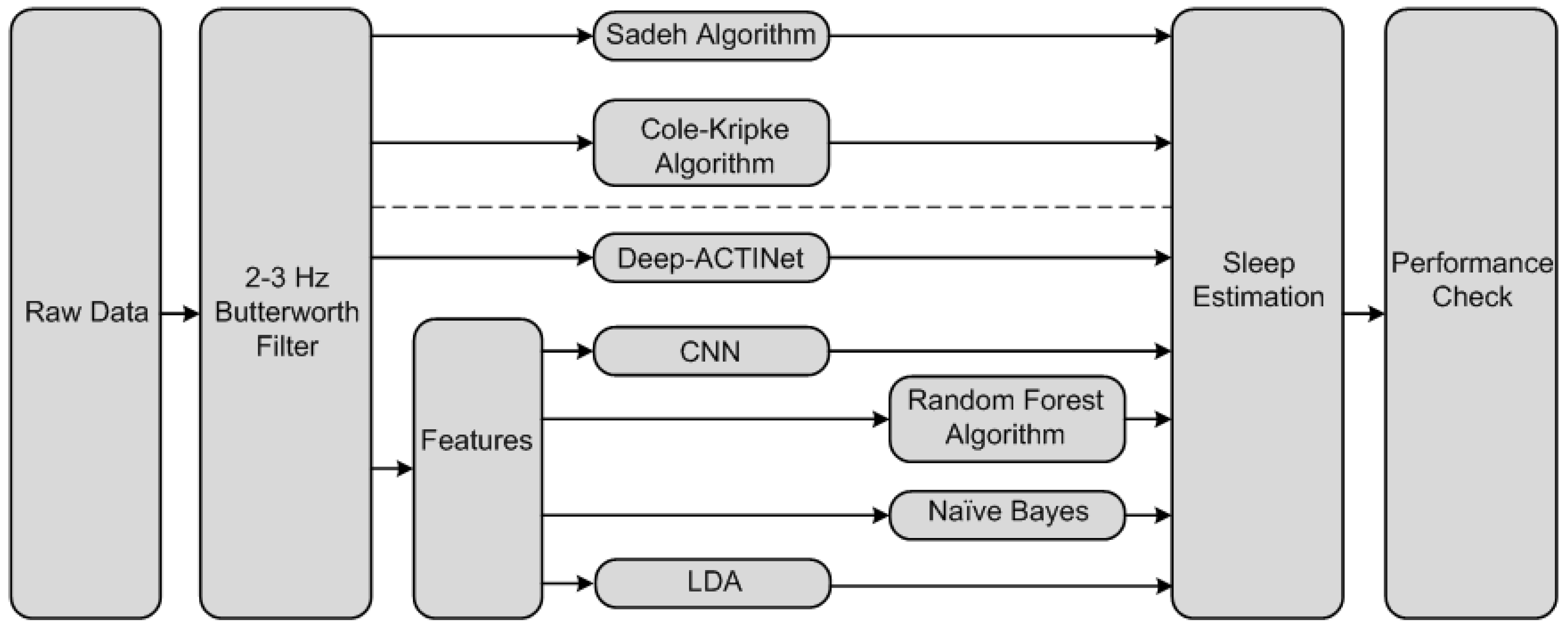
Traditional sleep detection algorithms and three conventional machine learning methods were compared with the proposed algorithm (deep learning architecture using wrist actigraphy (Deep-ACTINet model)), which is described in Section 2.3, based on the two ground truths of diary bed and diary sleep labels, as shown in Figure 1. Additionally, a feature based CNN architecture was also designed and tested to investigate the benefit of the end-to-end Deep-ACTINet model.

Figure 1 describes all seven methods implemented in this paper. The first two methods were traditional sleep detection algorithms using the Sadeh and Cole–Kripke algorithms. These traditional methods use activity count to score sleep-wake states. The third method was the proposed Deep-ACTINet, which processes raw data input using one-dimensional CNN (1D CNN) and LSTM to extract the abstract features from the local time slot and solve the long time lag problem. The other methods apply conventional feature engineering to get the features, where 10 features were extracted from the input data. Unlike Deep-ACTINet, the CNN model uses the extracted features as the input instead of raw data. Random forest, naive Bayes and LDA were also employed as conventional machine learning approaches to score the sleep-wake states.

1.2. Traditional Sleep Detection Methods

1.2.1. Sadeh Algorithm

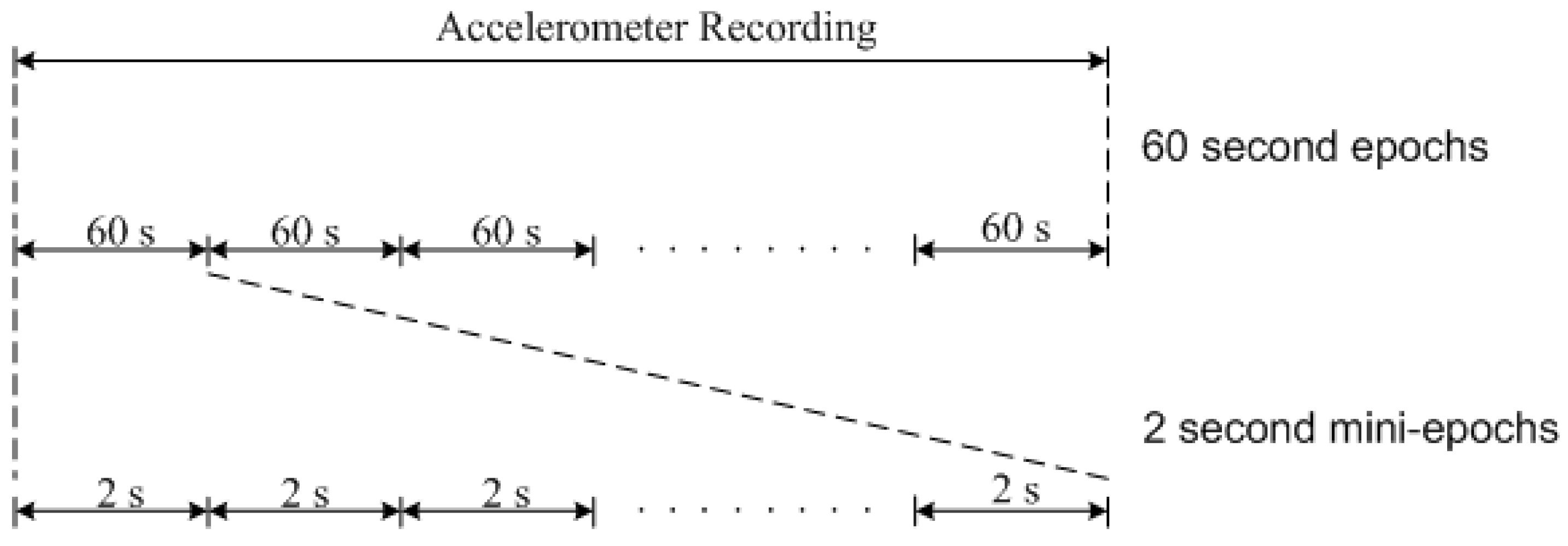
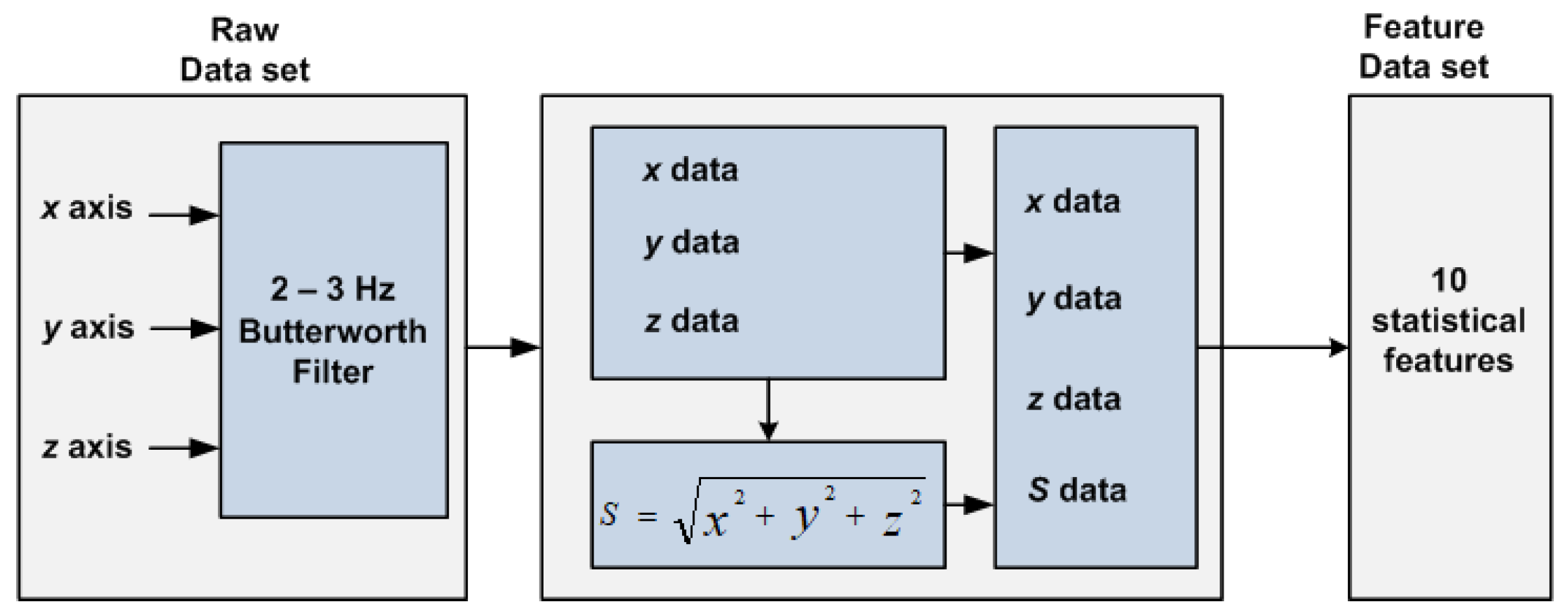
A conventional Sadeh algorithm using the accelerometer data was used in this simulation [12,35] with the purpose to identify the asleep and awake states. This method extracts features based on an activity count, which is the number of zero-crossing points during a 2 s mini-epoch. In this algorithm, the zero-point threshold was modified to 0.02 in order to deal with hardware noise. The process of the activity count is illustrated in Figure 2.

The three-axis accelerometer data were filtered using a Butterworth filter at a frequency of 2–3 Hz. The length of the data was then segmented into 60 s epochs. In a 60 s epoch, the amplitude of the data was calculated using the square root of the three-axis data. The activity was counted when the amplitude of the squared root of the accelerometer data crossed the threshold. A 60 s epoch was segmented into 2 s mini-epochs. Finally, the activity count of each 60 s epoch was counted based on the maximum value of activity in all 2 s mini-epochs.

Four statistical Sadeh features were then employed in the activity count to generate the features of sleep-wake scoring [12]. These features were the mean of a 5 min window, the standard deviation of a 6 min preceding window, the natural logarithm of the activity count number during the scored epoch + 1 (LOG-Act), and the number of epochs that had activity levels between 50 and 100, including the current epoch (NAT). Finally, a linear regression process was applied to produce a classification output that was like the following.

$$Y^{{}^{\prime }}=a+bX$$

(1)

$$a={\displaystyle \frac{{\sum }_{i=1}^N{Y}_i-b{\sum }_{i=1}^N{X}_i}{N}}$$

(2)

$$b={\displaystyle \frac{N\left({\sum }_{i=1}^N{X}_i{Y}_i\right)-\left({\sum }_{i=1}^N{X}_i\right)\left({\sum }_{i=1}^N{Y}_i\right)}{N{\sum }_{i=1}^N{X}^2-{\left({\sum }_{i=1}^N{X}_i\right)}^2}}$$

(3)

where $Y^{{}^{\prime }}$ represents the predicted value by the output of linear regression. X is input data, and a and b are the constant value and regression coefficient of the linear model, respectively.

1.2.2. Cole–Kripke Algorithm

The Kripke algorithm is a traditional sleep estimation algorithm that was proposed by Cole et al. [13]. It can distinguish asleep states from awake states automatically using movement information from a wristband accelerometer sensor system. Using the fifth order Butterworth filter, The accelerometer data were filtered into 2–3 Hz. After the filtering process, the activity count was calculated. There are several methods for the estimation of the activity count, including MAXACT, SUMACT, zero-crossing mode (ZCM), time-above-threshold (TAT), and proportional-integrating mode (PIM) [13,36,37]. According to a recent study [38], the PIM activity count method, compared to the other methods, yields the highest accuracy performance. This procedure was then followed by the feature extraction, wherein the extracted features are summated after their own predefined weights are multiplied. If this value exceeded a threshold, the sample was considered to be in an awake state. If not, it was considered to be in an asleep state.

1.3. Conventional Machine Learning Methods

1.3.1. Feature-Based CNN

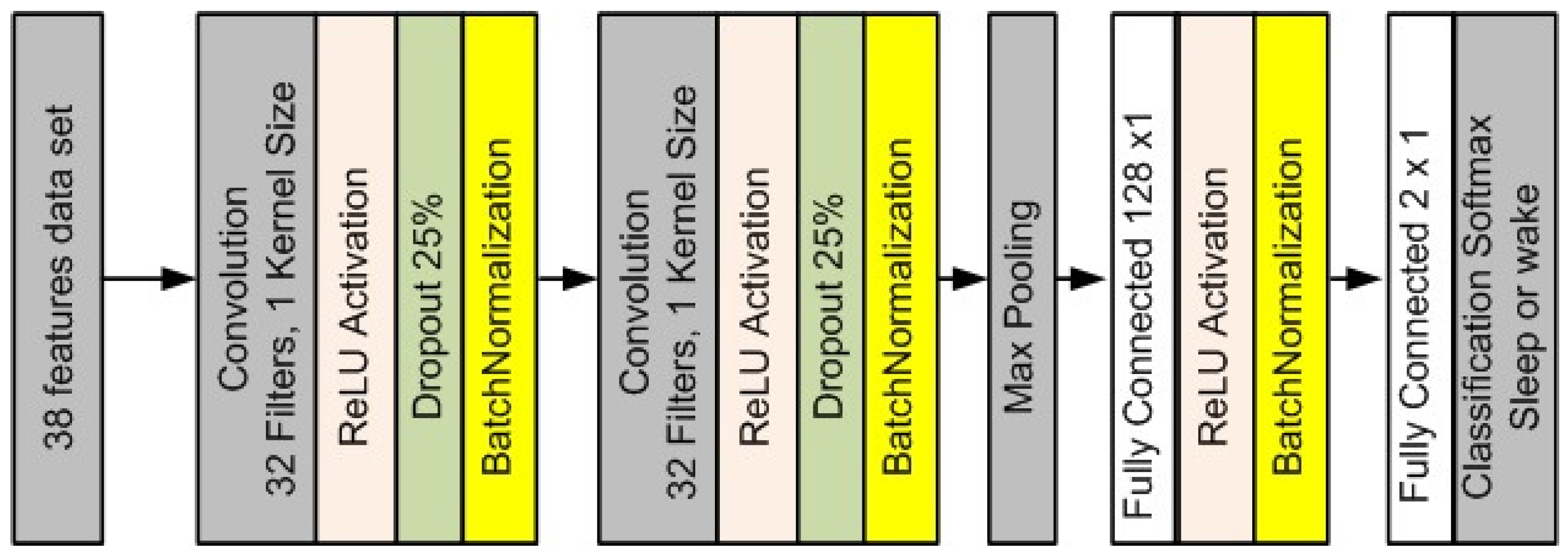
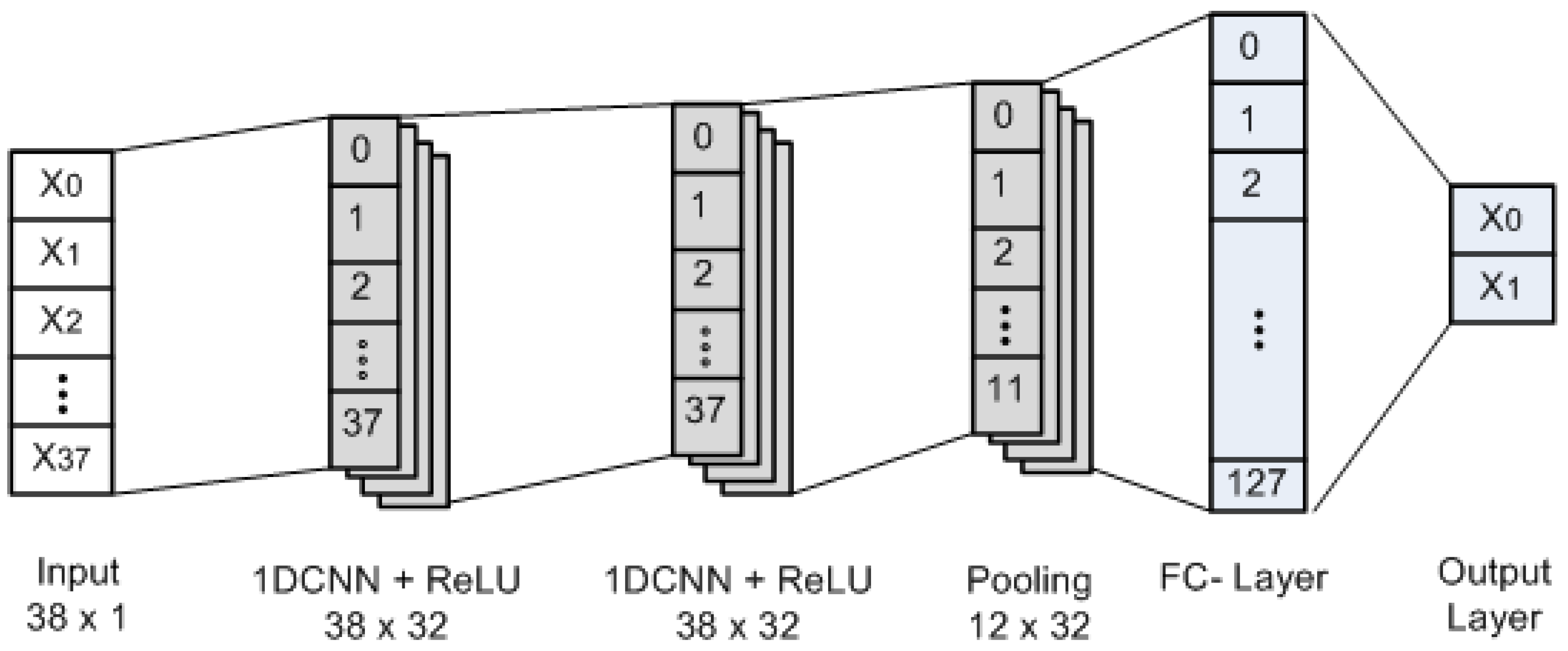
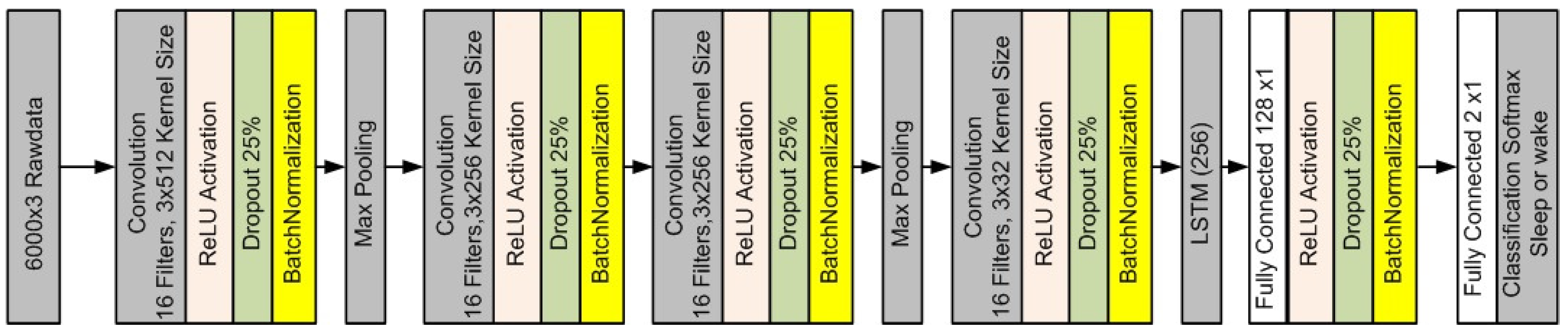
A CNN architecture based on extracted feature input, where the features are obtained via traditional feature engineering methods in time and frequency domains, was constructed. Two layers of a 1D convolution, consisting of 32 convolutional filters with a small receptive field, the ReLU activation function, dropout, and batch normalization, were designed. As shown in Figure 3, max pooling was performed to reduce the dimensions of the feature map. The stack of the convolution layers was followed by two fully connected (FC) layers, where the first layer was connected to a ReLU activation function and batch normalization, and the second FC layer of size two, corresponding to the number of classes, was followed by a softmax classifier for the final prediction.

1.3.2. Random Forest

Random forest (RF) is an ensemble learning method for classification and regression tasks [39,40]. RF, including an additional layer of randomness for bootstrap aggregation, was proposed by Breiman et al. (2001). This machine learning algorithm consists of many decision trees, where each node is divided using the best among the subsets of predictors randomly selected at the node. The results are decided by a majority vote of the decision trees [39,41,42]. This somewhat counterintuitive strategy performs quite well compared to several other classifiers, such as discriminant analysis and support vector machines, and is robust against overfitting [39].

1.3.3. Naive Bayes

The naive Bayes classifier is based on Bayes’ rule, where it supposes that all features of samples are independent of each other in the context of the class. Owing to this so-called “naive Bayes assumption”, the parameters for each feature could be learned separately, and this obviously simplifies the learning procedure, especially when there is a large number of attributes [43]. The naive Bayes classifier has been used to predict sleep stages for the diagnosis of health condition using EOG, EEG, and submental-EMG [44].

$$P\left(Y\right|X)={\displaystyle \frac{P\left(X\right|Y\left)P\right(Y)}{P\left(X\right)}},$$

(4)

where $P\left(Y\right|X)$ is a posterior probability function that represents the probability of the class Y given the input parameter X. Likelihood function $P\left(X\right|Y)$ represents the probability of the observed X given a set of class Y, while $P\left(Y\right)$ represents a prior probability function.

1.3.4. Linear Discriminant Analysis

Linear discriminant analysis (LDA) is a commonly used technique for data classification and dimensionality reduction. This method maximizes the ratio of between-class variance to within-class variance in the dataset, thus guaranteeing maximal separability. LDA does not change the location of original datasets, but only tries to ensure more class separability and draws a decision boundary between the given classes [18,45].

In this study, we applied a deep neural network to accelerometer data from actigraphy, using the convolutional neural network combined with LSTM model, which could extract features from raw data without any handcrafted software engineering approaches. This method could be effective for the nonstationary actigraphy data because of its data driven way of building a model by learning the raw data. In addition, the combination of CNN and LSTM was designed to extract features from local time slots and estimate the relationship across the features. The advantage of the proposed model was demonstrated via a benchmark test between handcrafted feature based CNN, data driven DNN architectures, and conventional actigraphy sleep scoring algorithms. Lastly, the explanation for the proposed DNN model is provided via a comparison between the features of the DNN and of traditional methods [46,47,48].

This paper is organized into five sections: Section 1.1, Section 1.2 and Section 1.3 describe the benchmark test using traditional sleep scoring algorithms and conventional machine learning methods. Section 2 presents the deep learning architectures of the proposed method, CNN + LSTM. Section 3 explains the details of our research background and evaluation method. Section 4 presents the results of the experiment. Finally, in Section 5, we provide some concluding remarks regarding this study.

2. Deep Learning Architectures

2.1. Convolutional Neural Network

Recently, a deep learning architecture named convolutional neural network (CNN), inspired by the neurobiological structure in the visual cortex of mammals, was introduced. Over the last few years, CNNs have accomplished state-of-the-art performance in various domains such as computer vision. CNN includes repetitive filters applied to local time slots [33], which yield high level abstract features, and after this process, which is called convolution, a pooling process is performed to find the most significant abstract features. This design of CNN results in fewer parameters than those of its fully connected network and therefore has a strong generalization capability for target prediction tasks [33]. This procedure is potentially followed by one or more fully connected layers. In classification problems, such as the sleep scoring and image recognition, the last layer of CNNs is usually a softmax layer. CNN are trained using a repeated optimization approach with the backpropagation algorithm [24]. Another advantage of CNN is its ability to prevent hand designed input features from being obtained from a specific problem [49]. Compared with many deep learning models, the architecture of CNN could design optimal time invariant local feature extractors from input data [50]. Two methods utilizing one-dimensional CNN for detecting sleep-wake patterns from actigraphy motor sensor data are presented in this paper: the first method is a feature based CNN, which has a number of channels, whereas the second method is based on an end-to-end data driven approach, which is combined with a long short term memory (LSTMs) recurrent neural network.

Figure 4 illustrates the structure of the 1D CNN receiving data in 38 × 1 dimensions as an input. Thirty two filters with a 1 × 1 kernel size were applied for the first two layers, which produced a 38 × 32 feature map by the convolution of the input data, and the same process was implemented in the second layer. A pooling layer with a kernel size of three was employed with a stride of three to prevent overfitting issues after the convolutional processes, where the output of this layer was a feature map with size 12 × 32. A fully connected layer was used to make high level feature vector for the sleep staging from the output of the previous layer. The softmax was utilized as an activation function for the final classification of the sleep stages. Algorithm 1 is the pseudocode of the CNN example implemented in this simulation. This architecture employs dropout and batch normalization to solve the overfitting problem and accelerate data processing. During the learning process, a 0.001 learning rate with 20 epoch and a mini-batch size of 64 were used.

Algorithm 1 CNN architecture pseudocode

$1:$  $\mathbf{CNN}(trainX,trainY,testX,testY,learningrate=0.001,epoch=20,batchsize=64):$ $2:$     $inputs=shape(datapoints,channels)$ $3:$     $model\leftarrow Conv1D(filters=32,kernels=1,activation=ReLU)\left(input\right)$ $4:$     $model\leftarrow Dropout\left(0.25\right)\left(model\right)$ $5:$     $model\leftarrow BatchNormalization\left(\right)\left(model\right)$ $6:$     $model\leftarrow Conv1D(filters=32,kernels=1,activation=ReLU)\left(model\right)$ $7:$     $model\leftarrow Dropout\left(0.25\right)\left(model\right)$ $8:$     $model\leftarrow BatchNormalization\left(\right)\left(model\right)$ $9:$     $model\leftarrow MaxPooling\left(model\right)$ $10:$   $model\leftarrow Flatten\left(\right)\left(model\right)$ $11:$   $model\leftarrow Dense(neurons=128,activation=ReLU)\left(model\right)$ $12:$   $model\leftarrow BatchNormalization\left(model\right)$ $13:$   $model\leftarrow Dense(neurons=2,activation=softmax)\left(model\right)$ $14:$   $model.compile(loss=BinaryCrossEntropy,optimizer=Adam,learningrate)$ $15:$   $model.fit(trainX,trainY,epoch,batchsize)$ $16:$   $Accuracy=model.evaluate(testX,testY)$ $17:$   $\mathbf{return}Accuracy$

2.2. Long Short Term Memory

Long short term memory (LSTM), a complicated type of deep learning architecture published in 1997 by Hochreiter and Schmidhuber [51], includes memory for representing temporal dependencies in time sequential problems. LSTM extends a deep recurrent neural network (RNN) with memory blocks containing memory cells, instead of recurrent units, to ease the learning of temporal relationships when there are long time delays between events. The memory cell has three different gates: an input gate, a forget gate, and an output gate. These gates decide which operation is to be performed, such as write (input gate), reset (forget gate), or read (output gate). In particular, the forget gate adjusts the internal value of the cell before adding it as an input to the cell using self-recurrent connection, therefore suitably resetting or forgetting the cell’s memory [52]. Additionally, a modern LSTM architecture includes peephole connections from its inner cells to the gates in order to learn exact timing of the outputs [53]. The activation functions of the LSTM units are operated in the same way as those in RNNs [51], and the hidden value of an LSTM cell is updated at each time step. LSTM has recently achieved great success in time series analysis, for example in speech recognition [54] and language translation tasks [55].

Figure 5 shows an LSTM in a single neuron. The sequential data $X_t$ is fed into LSTM and then concatenated with the previous hidden state $h_{t-1}$ after linear combination. The first sigmoid activation function is responsible for determining how much old memory $C_{t-1}$ will be used for the current state. The variable $j_t$ represents the output from the old memory that will be used for the current state. The second sigmoid activation function is responsible for determining how much memory will be used from new memory $s_t$. The current memory $C_t$ is calculated by the equation $C_t=f_t\ast C_{t-1}+u_t\ast s_t$. That is a combination of old memory and current information.

Algorithm 2 is the pseudocode of LSTM that receives data with a size of 12 as an input, whose goal is a binary classification. An LSTM layer was designed with 0.25 dropout solving the overfitting problem, which accelerates data processing. A fully connected layer with softmax activation function was used for the classification. During the learning process, a 0.001 learning rate with 20 epochs and mini-batch size of 64 were used.

Algorithm 2 LSTM architecture pseudocode

$1:$  $\mathbf{LSTM}(trainX,trainY,testX,testY,learningrate=0.001,epoch=20,batchsize=64):$ $2:$     $inputs=shape(features=12)$ $3:$     $model\leftarrow LSTM(hiddensize=32)\left(input\right)$ $4:$     $model\leftarrow Dropout\left(0.25\right)\left(model\right)$ $5:$     $model\leftarrow Dense(neurons=2,activation=softmax)\left(model\right)$ $6:$     $model.compile(loss=BinaryCrossEntropy,optimizer=Adam,learningrate)$ $7:$     $model.fit(trainX,trainY,epoch,batchsize)$ $8:$     $Accuracy=model.evaluate(testX,testY)$ $9:$     $\mathbf{return}Accuracy$

2.3. Deep-ACTINet

In this study, Deep-ACTINet, which is based on a hybrid of CNN and LSTM (CNN + LSTM), was designed to analyze the three-axis accelerometer data from a wristband sensor for sleep-wake detection, as illustrated in Figure 6. CNN extracts features from the signal pattern, the temporal sequence of which is looked into using the LSTM architecture. Raw accelerometer data are fed into the input neurons, and the network learns the morphological and temporal patterns of the data to group the sleep and wake states. In an end-to-end data driven way, the dimension of the data is 6000 × 3, consisting of 3 channel data in a 60 s epoch sampled at 100 Hz in a learning network model. We used three layers of convolution with the same numbers of filters and employed the rectified linear unit (ReLU) as the activation function. Dropout of 0.25 was used as a regularization mechanism to deal with the overfitting problem. Batch normalization was used to accelerate training by normalizing the output activation of the previous layer. At the end of the layer, a pooling process was employed to reduce the size of the feature map. We chose max pooling as a mechanism in the pooling process. Reducing the size of the feature map is equivalent to reducing the number of parameters to be processed in the next layer, which could make the training process faster. The output of the first convolution layer would be the input of the second layer, and so on. The details of the Deep-ACTINet architecture are described in Figure 6. After the convolution layer, the LSTM layer was employed to process the feature map from the previous CNN layers, and at the end, a fully connected layer with the softmax function [56] was used to infer the sleep or wake state. Binary cross-entropy was employed as an objective function, and the Adam optimizer was used to optimize the weight parameters of the network.

Algorithm 3 Deep-ACTINet architecture pseudocode

$1:$  $\mathbf{Deep}\text{-}\mathbf{ACTINet}(trainX,trainY,testX,testY,learningrate=0.001,epoch=20,batchsize=64):$ $2:$     $inputs=shape(datapoints,channels)$ $3:$     $model\leftarrow Conv1D(filters=16,kernels=512,activation=ReLU,stride=2)\left(input\right)$ $4:$     $model\leftarrow Dropout\left(0.25\right)\left(model\right)$ $5:$     $model\leftarrow BatchNormalization\left(\right)\left(model\right)$ $6:$     $model\leftarrow MaxPooling\left(model\right)$ $7:$     $model\leftarrow Conv1D(filters=16,kernels=256,activation=ReLU,stride=2)\left(model\right)$ $8:$     $model\leftarrow Dropout\left(0.25\right)\left(model\right)$ $9:$     $model\leftarrow BatchNormalization\left(\right)\left(model\right)$ $10:$   $model\leftarrow Conv1D(filters=16,kernels=256,activation=ReLU,stride=2)\left(model\right)$ $11:$   $model\leftarrow Dropout\left(0.25\right)\left(model\right)$ $12:$   $model\leftarrow BatchNormalization\left(\right)\left(model\right)$ $13:$   $model\leftarrow MaxPooling\left(model\right)$ $14:$   $model\leftarrow Conv1D(filters=16,kernels=32,activation=ReLU,stride=2)\left(model\right)$ $15:$   $model\leftarrow Dropout\left(0.25\right)\left(model\right)$ $16:$   $model\leftarrow BatchNormalization\left(\right)\left(model\right)$ $17:$   $model\leftarrow LSTM(hiddensize=256)\left(input\right)$ $18:$   $model\leftarrow Dense(neurons=128,activation=ReLU)\left(model\right)$ $19:$   $model\leftarrow Dropout\left(0.25\right)\left(model\right)$ $20:$   $model\leftarrow BatchNormalization\left(\right)\left(model\right)$ $21:$   $model\leftarrow Dense(neurons=2,activation=softmax)\left(model\right)$ $22:$   $model.compile(loss=BinaryCrossEntropy,optimizer=Adam,learningrate)$ $23:$   $model.fit(trainX,trainY,epoch,batchsize)$ $24:$   $Accuracy=model.evaluate(testX,testY)$ $25:$   $\mathbf{return}Accuracy$

The details of the Deep-ACTINet architecture are shown in Figure 6 and Algorithm 3. This architecture was built using four 1D CNNs with the same number of filters, 16. The shape of the input was a 6000 × 3 matrix, which means 6000 time data points and three channels. In the first convolution layer, a 512 kernel size was applied to operate convolution with raw input data. A 256 kernel size was used in the second and third convolution layer followed by a 32 kernel size in the last convolution layer. ReLU was used as the activation function in each convolution layer. After three CNN layers, an LSTM layer was applied to deal with sequential feature map from the previous layer. This architecture employed dropout and batch normalization to solve the overfitting problem and accelerate data processing. At the end of the model, a fully connected layer with two neurons was employed for classification. This neuron number represented the number of classes (sleep and wake). For the fitting process, a 0.001 learning rate with 20 epochs and a batchsize of 64 were used. All hyper parameters were manually adjusted while checking the loss function and performance.

3. Methods

3.1. Accelerometer Device

The GT3X (Actilife, USA), which can record wrist movements using an accelerometer sensor, was used for the experiment. It has a sensitivity of 3 mg/LSB, a dynamic range from −6 G to 6 G, and a 12-bit analog-to-digital converter (AD converter). The sampling rate of the GT3X can be modified from 30 Hz to 100 Hz, which is enough for detecting human movements.

3.2. Experiments

Ten healthy volunteers, composed of three females and seven males, participated in the experiment for this research. Each subject, while sleeping at his or her home, underwent movement data recordings using an accelerometer band around the non-dominant wrist. The data were recorded with a sampling rate of 100 Hz, both when the subject was asleep and when the subject was awake. All subjects were required to write their in-out times for bed and their sleep-wake times. Afterward, the accelerometer data were manually scored corresponding to these sleep diaries. For this experiment, we marked two types of labels: diary sleep label, which indicated whether the subject was asleep or not, and diary bed label, which indicated whether the subjects were lying in bed or not.

Table 1. Number of epochs corresponding to the sleep diary labels and physical information on the subjects.

Subject	Awake Epoch	Sleep Epoch	Total	Sex	Height	Weight	BMI
Index	(Bed, Sleep)	(Bed, Sleep)	Epoch		(cm)	(kg)	(kg/m${}^2$)
1	(7390, 7085)	(3020, 3325)	10,410	Male	174	80	26.42
2	(6250, 6007)	(4370, 4613)	10,620	Male	168	57	20.20
3	(7076, 6901)	(2835, 3010)	9911	Male	173	70	23.39
4	(12,273, 11,660)	(4902, 5515)	17,175	Female	158	48	19.23
5	(6531, 6104)	(3085, 3512)	9616	Male	170	69	23.88
6	(12,058, 11,918)	(3372, 3512)	15,430	Female	164	52	19.33
7	(8271, 7741)	(3170, 3700)	11,441	Male	168	62	21.97
8	(8551, 7997)	(4121, 4675)	12,672	Male	186	100	28.91
9	(5895, 5768)	(3050, 3177)	8945	Male	178	80	25.25
10	(10,764, 10,557)	(6150, 6357)	16,914	Female	168	50	17.72

outlines the physical and epoch information on each subject.

3.3. Preprocessing

The data were filtered using a fifth order Butterworth filter, the cut-off frequency of which was from 2 Hz to 3 Hz, to remove movement artifacts. The filtered accelerometer data were arranged into minute-by-minute epochs because the Kripke algorithm estimated the sleep states using a 60 s epoch.

3.4. Feature Extraction

Nine time domain features and one frequency domain feature were extracted from the accelerometer raw data recorded from the subjects. The process of feature extraction is illustrated in Figure 7. These feature extraction methods involved the mean, standard deviation, correlation, kurtosis, crest factor, skewness, zero-crossing, entropy, band energy, and spectral flux, as described in

Table 2. The 10 features in the time and frequency domains.

No	Feature	Equation	Description
1	Mean	$\overline{x}={\displaystyle \frac{1}{N}\sum _{n=1}^N}x\left(n\right)$	Total amount of accelerometer data x(n) with respect to the data length of an epoch (N).
2	Standard Deviation	$Std\left(x\right)=\sqrt{{\displaystyle \frac{1}{N-1}\sum _{n=1}^N}{(x\left(n\right)-\overline{x})}^2}$	Describing how spread out the accelerometer data are.
3	Correlation	$Corr(x,y)={\displaystyle \frac{1}{N-1}\sum _{n=1}^N}{\displaystyle \frac{(x_n-\overline{x})(y_n-\overline{y})}{Std\left(x\right)Std\left(y\right)}}$	Representing the relation between two components (x- and y-axis) of accelerometer data.
4	Kurtosis	$K\left(x\right)={\displaystyle \frac{E{(x-\overline{x})}^4}{Std{\left(x\right)}^2}}-3$	Tailedness of the probability distribution of real value x-axis accelerometer data using the 4th central moment, with respect to variance.
5	Crest Factor	$CF\left(x\right)=\frac{max\left(x\right(n\left)\right)}{\sqrt{{\displaystyle \sum _{n=1}^N}x{\left(n\right)}^2}}$	Indicating how extreme the peak of data is in the overall data by measuring the ratio of the maximum value of the data to the effective value of accelerometer data.
6	Skewness	$\gamma \left(x\right)=E\left[{\left({\displaystyle \frac{x-\overline{x}}{Std\left(x\right)}}\right)}^2\right]$	Measure of the asymmetry probability distribution of the accelerometer data x-axis to their mean.
7	Zero-Crossing	$ZCR\left(x\right)=\left||n\in N|(2\le n\ge N)\wedge \left(a\right(n)·a(n-1\left)\right)\right|$	Total number of zero-crossings in accelerometer data.
8	Entropy	$S\left(x\right)=-{\displaystyle \sum _k}{p}_x\left(k\right)ln\left(p_x\left(k\right)\right)$	Total probability mass function of x-axis data in accelerometer data.
9	Band Energy	$BE\left(t\right)=\frac{{\displaystyle \sum _{n=1}^N}{x}^{{}^{\prime }}\left(n\right)}{{\displaystyle \sum _{n=1}^N}x\left(n\right)}$	Normalized energy sub-band with respect to the total energy of the signal. $x^{{}^{\prime }}$ is the sub-band signal (2–3 Hz).
10	Spectral Flux	$SF\left(t\right)={\displaystyle \sum _{n=2}^N}{(x_t\left(n\right)-x_{t-1}\left(n\right))}^2$	Total difference between the successive data of accelerometer data.

. These methods were calculated using the squared root data and the three-axis data, producing 38 feature datasets. The correlation and zero-crossing could not be calculated using the single square root signal.

3.5. Evaluation Method

The performance of the model was evaluated using the following three scoring criteria, that is classification accuracy, precision, and recall. The accuracy or agreement rate was calculated as follows:

$$Agreementrate=\frac{TP+TN}{TP+TN+FN+FP}$$

(5)

where TP, TN, FP, and FN represent the true positive, true negative, false positive, and false negative, respectively. Recall or sensitivity refers to the TP rate among all the positive samples [57]. It is formulated as:

$$Recall=\frac{TP}{TP+FN}.$$

(6)

The precision or positive predictive value is the TP rate among all the predicted positive samples [57]. It is calculated as:

$$Precision=\frac{TP}{TP+FP}.$$

(7)

To compare the validities of the models, 10-fold cross-validation was performed for Deep-ACTINet and all the other benchmark test methods using an intersubject test/train methodology, wherein 9 subject datasets were used in training and the remaining dataset was tested. Finally, all the results obtained using the different classifiers were tested using the one tailed paired t-test to check the significance of the differences between them.

4. Results

The three-axis accelerometer data recorded during the experiment were classified using these methods that have been mentioned earlier: 2 traditional Sadeh and Cole–Kripke algorithms, 3 conventional machine learning approaches, and 2 deep neural network architectures with or without the feature engineering. Ten-fold cross-validation was performed to evaluate the performance of the applied methods over the ten subjects.

The average accuracy, recall, and precision of the sleep detection results based on the diary bed label are shown in

Table 3. Classification performance of asleep and awake states based on the diary bed label.

Methods	Accuracy (%)	Recall (%)	Precision (%)
Sadeh	84.91 ± 3.80	89.03 ± 6.41	89.19 ± 3.74
Cole–Kripke	80.30 ± 4.13	79.38 ± 6.48	90.73 ± 5.25
Deep-ACTINet	89.65 ± 3.67	92.99 ± 4.32	92.09 ± 2.11
Feature-Based CNN	84.14 ± 3.88	90.40 ± 3.13	87.08 ± 3.55
Random Forest	85.60 ± 4.06	91.06 ± 6.30	87.71 ± 2.34
Naive Bayes	81.43 ± 7.51	86.21 ± 9.72	86.72 ± 2.99
LDA	82.78 ± 2.16	87.54 ± 3.65	86.93 ± 3.05

, which includes their standard deviations. The proposed model, Deep-ACTINet, produced the best classification performance, with the values of 89.65% for accuracy, 92.99% for recall, and 92.09% for precision, based on the diary bed label.

Table 4. Classification performance of asleep and awake states based on the diary sleep label.

Methods	Accuracy (%)	Recall (%)	Precision (%)
Sadeh	84.18 ± 4.06	87.21 ± 7.02	87.74 ± 3.52
Cole–Kripke	80.19 ± 4.37	80.43 ± 6.86	88.28 ± 5.10
Deep-ACTINet	88.77 ± 3.97	92.96 ± 5.03	90.39 ± 2.38
Feature-Based CNN	83.79 ± 4.18	90.31 ± 2.64	85.89 ± 4.03
Random Forest	84.94 ± 3.85	91.92 ± 6.41	86.15 ± 2.16
Naive Bayes	80.49 ± 7.04	87.54 ± 9.67	83.60 ± 3.52
LDA	82.52 ± 2.09	87.25 ± 2.96	86.45 ± 2.58

presents the average of accuracy, recall, and precision for the diary sleep label. In this case, Deep-ACTINet also outperformed the other methods, with the values of 88.77% for accuracy, 92.96% for recall, and 90.39% for precision. Not only was the value of scoring parameters the highest, but the standard deviation was also relatively smaller than the others.

It was confirmed that the average performance on the diary bed label was better than the average performance on the diary sleep label. That was because the subjects lying in bed, but not sleeping could be interpreted as sleep states by a classifier using an accelerometer.

Acc.DBL, Acc.DSL, Rec.DBL, Rec.DSL, Pre.DBL and pre.DSL represent the accuracy, recall, and precision, respectively, of the diary bed label and the diary sleep label, respectively. For rigor, the differences in the accuracy, recall, and precision between Deep-ACTINet and the other methods were also investigated using the one tailed paired sample t-test, as shown in

Table 5. Student’s t-test between the conventional methods and Deep-ACTINet. Acc, accuracy; Rec., recall; Pre., precision; DBL, diary bed label; DSL, diary sleep label.

Methods	Acc.DBL	Acc.DSL	Rec.DBL	Rec.DSL	Pre.DBL	Pre.DSL
Sadeh	0.0190 ${}^{*}$	0.0320 ${}^{*}$	0.1680	0.0490 ${}^{*}$	0.1460	0.1750
Cole–Kripke	0.0040 ${}^{**}$	0.0050 ${}^{**}$	0.0010 ${}^{**}$	0.0030 ${}^{**}$	0.2890	0.1530
Feature based CNN	0.0060 ${}^{**}$	0.0190 ${}^{*}$	0.1630	0.1660	0.0080 ${}^{**}$	0.0240 ${}^{*}$
Random Forest	0.0470 ${}^{*}$	0.0650	0.4210	0.6930	0.0040 ${}^{**}$	0.0050 ${}^{**}$
Naive Bayes	0.0001 ${}^{**}$	0.0001 ${}^{**}$	0.0140 ${}^{*}$	0.0410 ${}^{*}$	0.0001 ${}^{**}$	0.0001 ${}^{**}$
LDA	0.0020 ${}^{**}$	0.0040 ${}^{**}$	0.0480 ${}^{*}$	0.0600	0.0001 ${}^{**}$	0.0020 ${}^{**}$

${}^{*}p<0.05$; ${}^{**}p<0.01$.

. Overall, it could be seen that the performance improvements by Deep-ACTINet were statistically significant, with p-values less than 0.05 or 0.01.

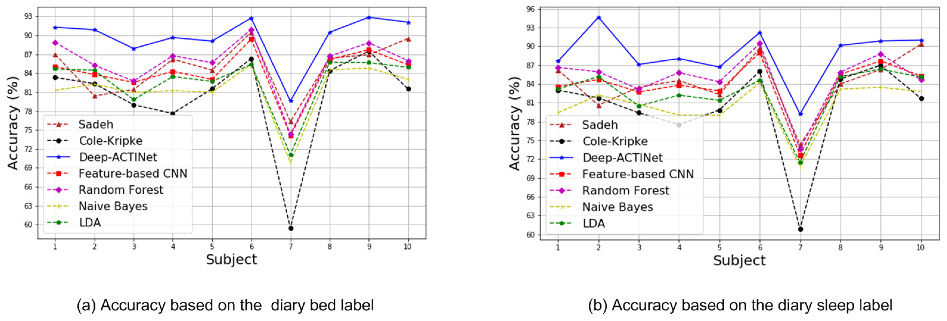
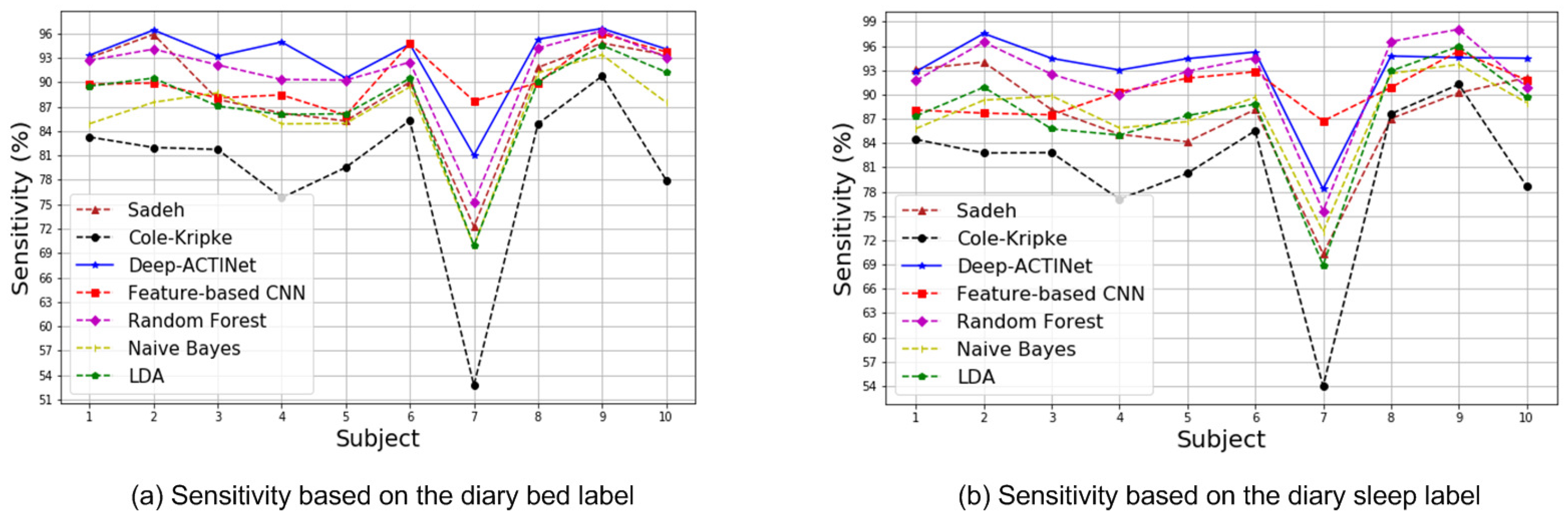
Figure 8, Figure 9 and Figure 10 show the results for the average accuracy, recall, and precision, respectively, of the subjects across 60 epochs. Note that Deep-ACTINet outperformed the other conventional classifiers based on both the diary bed labels and diary sleep labels, as shown in Figure 8. Subject 9 obtained the highest accuracy based on the diary bed labels, at 92.86%, whereas Subject 7 had the lowest, at 79.58%. Meanwhile, Subject 2 yielded the highest accuracy based on the diary sleep label, at 94.65%, and Subject 7 still had the lowest accuracy, at 79.21%.

Figure 9 illustrates the performance in terms of recall, emphasizing the TP rate among all the condition positive samples [57], that is sleep in this experiment. It was demonstrated that the proposed Deep-ACTINet produced the highest average recall value across all subjects based on both the diary bed labels (92.99%) and diary sleep labels (92.96%). Figure 9 also shows that Subject 7 had the lowest value of recall among all the subjects.

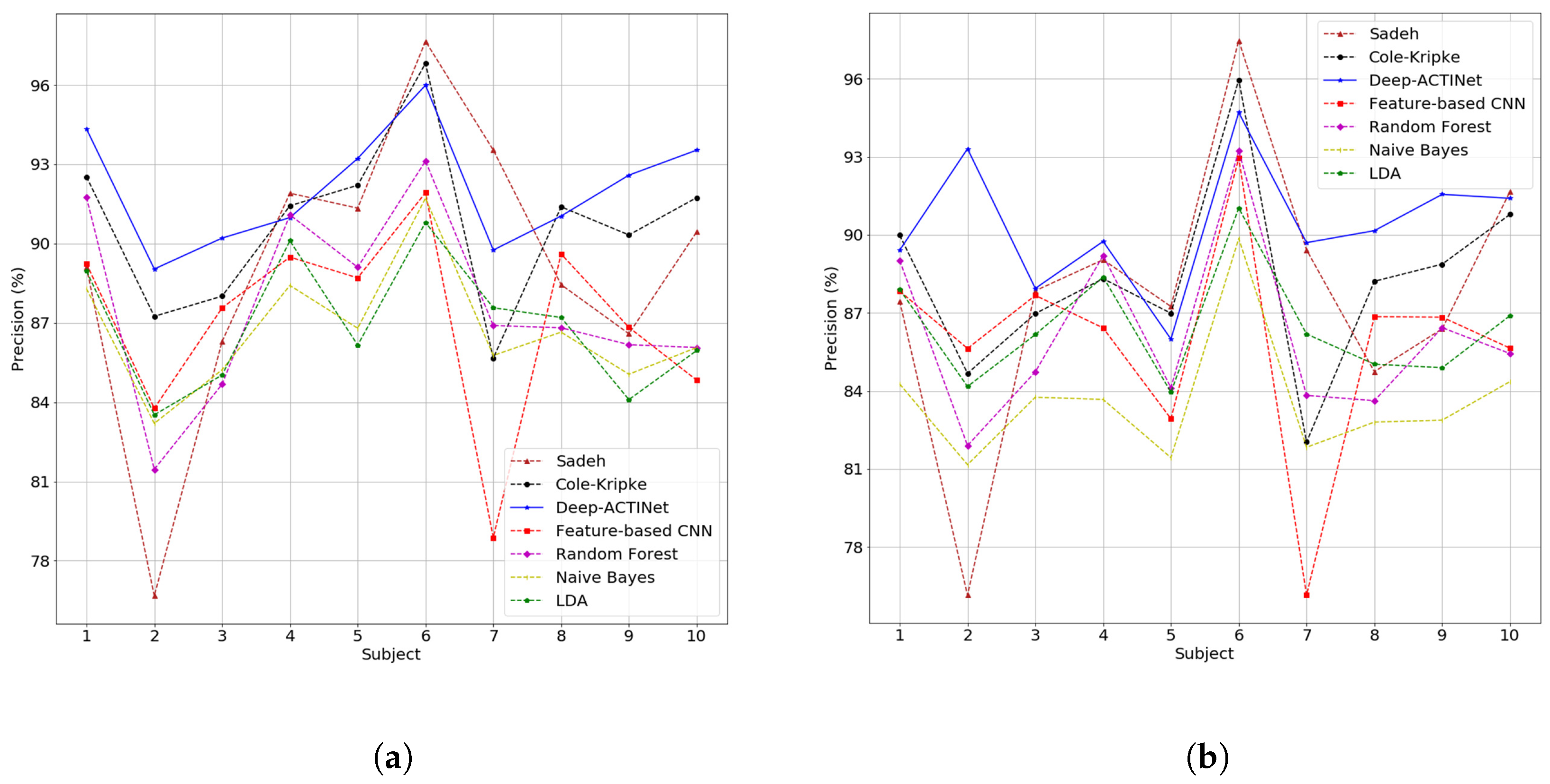
Figure 10 illustrates the performance in terms of precision, showing the TP rate among the predicted samples as a sleep state. Even for this metric, it was confirmed that Deep-ACTINet obtained the highest average precision based on both the diary bed labels (92.09%) and the diary sleep labels (90.39%). Even though the Sadeh algorithm reached the highest precision for Subject 6, overall, Deep-ACTINet was superior compared to the other methods.

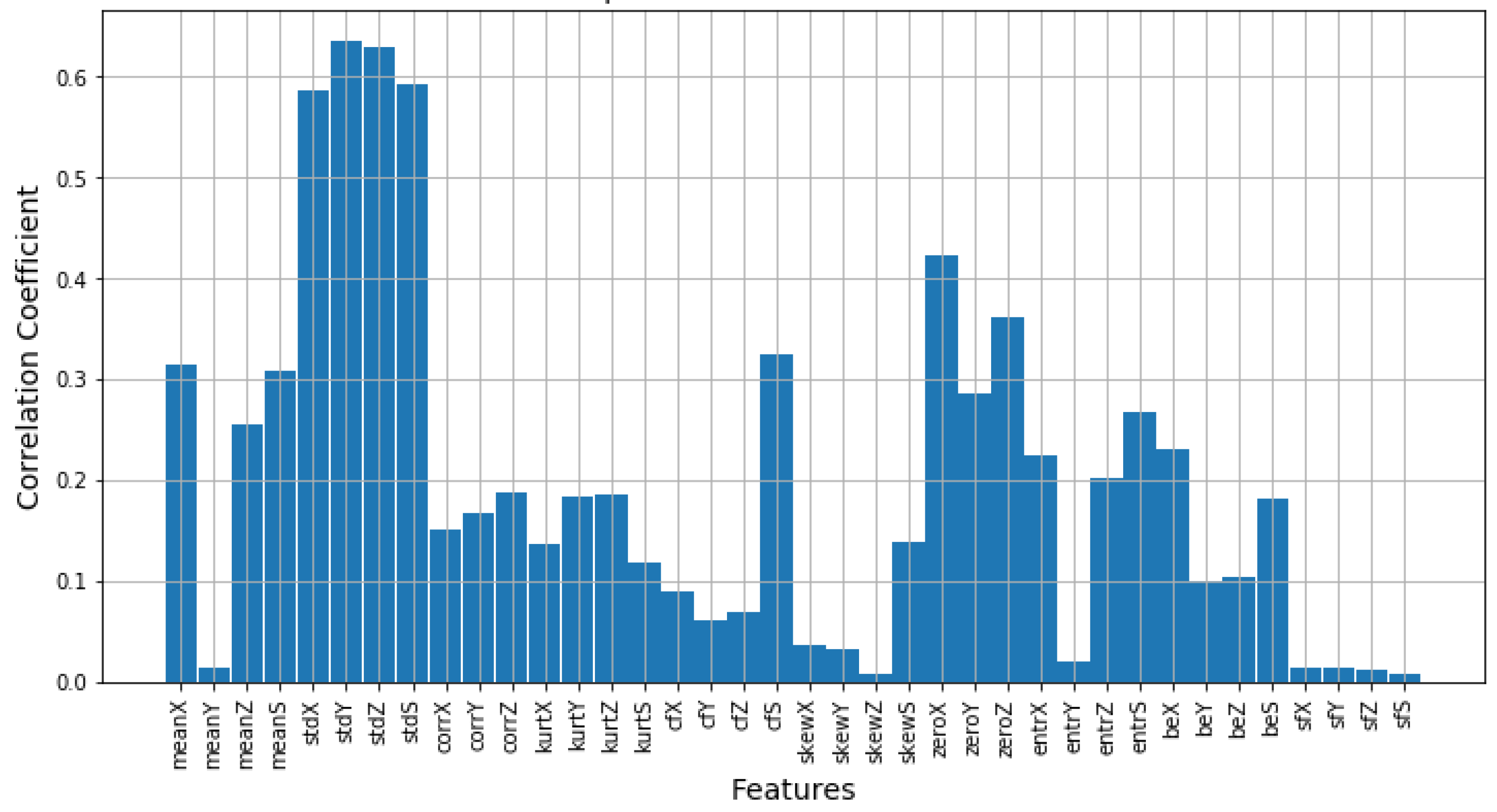
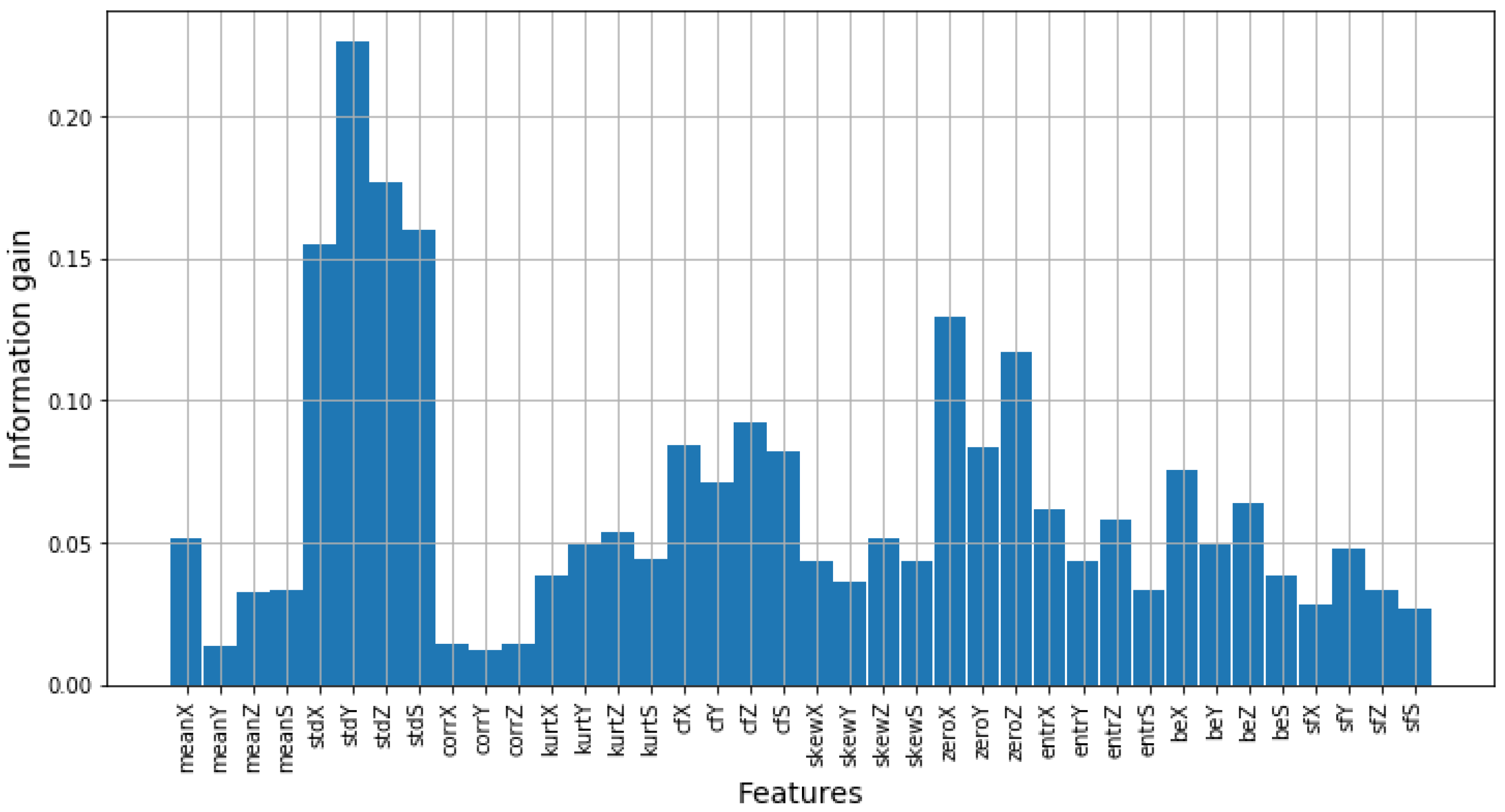
Additionally, the two neuron outputs of Deep-ACTINet just before the final classification output were thoroughly examined to compare their significance with those of the conventional feature engineering methods. Figure 11 describes the average correlation coefficients between the two outputs generated using Deep-ACTINet and the 38 conventional feature engineering features extracted in the time and frequency domains. The standard deviations of X, Y, Z, and S were noted to have strong correlations with the output of Deep-ACTINet, and the numbers of zero-crossing points of X and Z were also highly correlated with each other. In addition, the mutual information between the 38 features and class labels was calculated to find the effective features for sleep monitoring; the results are displayed in Figure 12, which shows the standard deviations of X, Y, Z, and S and the numbers of zero-crossing points of X and Z having large amounts of information. The visualization denotes that these features would be better than the others, and thus, these features could be used primarily for the classification [58]. Interestingly, the patterns of Figure 11 and Figure 12 are quite similar, from which we could infer that Deep-ACTINet extracted the most significant two outputs with highly efficient abstractions of the raw accelerometer signals to the sleep state. This characteristic could explain why the proposed deep learning architecture led to the improvement of classification performance.

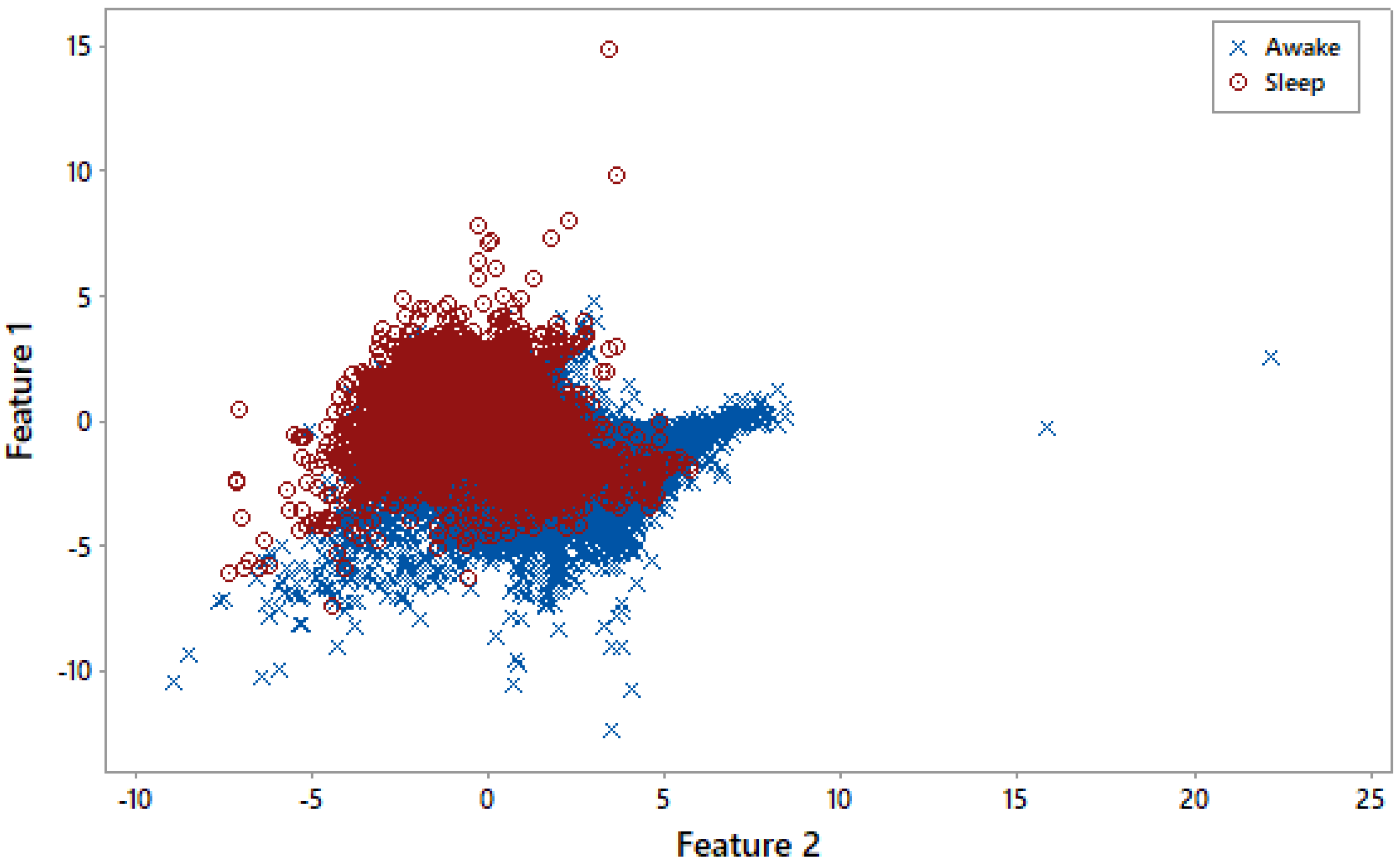
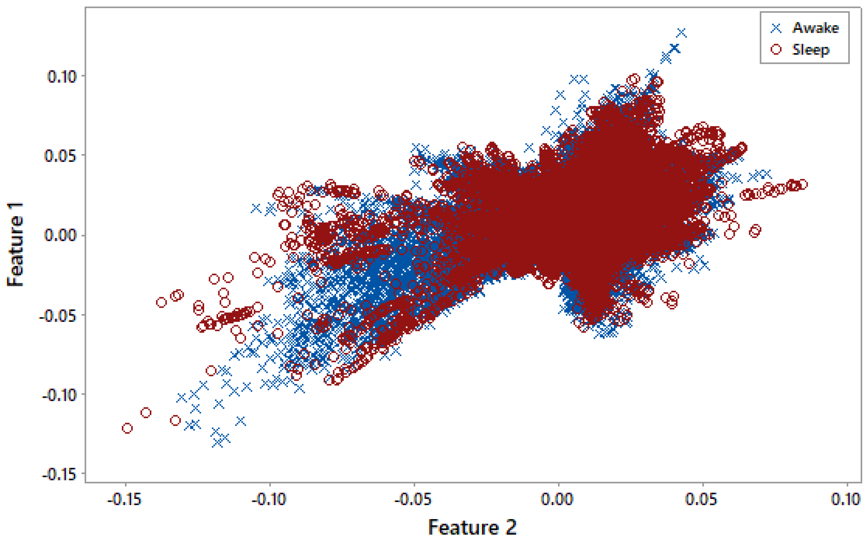
Figure 13 and Figure 14 depict the scatter plots of the last two outputs of Deep-ACTINet and feature based CNN, respectively, corresponding to the sleep states. These visualizations of the neuron outputs using the two deep learning models illustrate a little better separation of the end-to-end Deep-ACTINet outputs compared to that of the feature based CNN outputs, resulting in a higher classification rate. This result suggests that the data driven end-to-end architecture of Deep-ACTINet could be a more natural way to extract generic properties of the raw accelerometer data than the pre-defined model based feature engineering approaches.

There is also the relation between the last two outputs of the CNN + LSTM and those of the feature based CNN, where each sample was arranged according to the ground-truth. Because these two outputs were the inputs of the last softmax activation function, it could be expected that this negative relation could be seen more clearly, and each sample could be classified better. In Figure 13, it can be observed that sleep-wake states were divided much better than in Figure 14. These results support the notion that this end-to-end approach was more powerful than feature based CNN.

5. Discussion and Conclusions

In this study, several machine learning algorithms were tested for the estimation of asleep and awake states, compared with the traditional static model based algorithms, the Sadeh and Cole–Kripke algorithms. It is crucial to design a general model, by training machine learning algorithms, that is not overfitted to the training dataset that would otherwise limit it to working only for a few subjects. In order to avoid this overfitting problem, the machine learning algorithms in this research were designed via intersubject training, that is the training dataset did not include any test subject data. It was noted that the proposed deep learning model, Deep-ACTINet, produced generalized models that predicted the asleep and awake states with high accuracies, which was tested with a dataset that was not used in training. Remarkably, this proposed model significantly outperformed the most popular actigraphy algorithms, such as Sadeh and Cole–Kripke, suggesting that Deep-ACTINet could replace the current algorithms in wristband type wearable devices.

The sleep state classification based on two different sleep diaries, diary sleep and diary bed, was conducted in this experiment, and the performance based on the diary bed labels was better than the others. This is understandable considering the limitation of the accelerometer sensor, which only monitored the movement of a subject. Without any other physiological sensor, the accelerometer itself could not tell the difference between lying down without movement and actual sleeping. For future work, this would be solved with additional physiological data such as electroencephalogram (EEG), electrocardiogram (ECG), electromyogram (EMG), and so on.

This paper demonstrated an end-to-end data- driven deep learning model, Deep-ACTINet, that extracted the accelerometer features more efficiently than conventional feature engineering methods and eventually yielded higher sleep and wake separation rates compared with those of the conventional fixed model based and machine learning based algorithms. This was proven by the feature studies, where the neuron outputs by Deep-ACTINet were highly correlated with only the most significant conventional features. Furthermore, Deep-ACTINet was trained via intersubject training and thus yielded a general model that worked for all subjects. This result could suggest that sleep and wake detection algorithms in current actigraphy systems could be replaced by Deep-ACTINet.

References

1. Nofsinger, J.R.; Shank, C.A. DEEP sleep: The impact of sleep on financial risk taking. Rev. Financ. Econ. 2019, 37, 92–105. [Google Scholar] [CrossRef]
2. Beattie, L.; Kyle, S.D.; Espie, C.A.; Biello, S.M. Social interactions, emotion and sleep: A systematic review and research agenda. Sleep Med. Rev. 2015, 24, 83–100. [Google Scholar] [CrossRef] [PubMed]
3. Wenden, A.L. Case Studies in Sleep Neurology Common and Uncommon Presentations; Cambridge University Press: New York, NY, USA, 2010; Volume 3. [Google Scholar]
4. Carney, C.E.; Edinger, J.D.; Meyer, B.; Lindman, L.; Istre, T. Daily activities and sleep quality in college students. Chronobiol. Int. 2006, 23, 623–637. [Google Scholar] [CrossRef] [PubMed]
5. Engle-Friedman, M. The effects of sleep loss on capacity and effort. Sleep Sci. 2014, 7, 213–224. [Google Scholar] [CrossRef]
6. Prochazka, A.; Kuchynka, J.; Yadollahi, M.; Araujo, C.P.S.; Vysata, O. Adaptive segmentation of multimodal polysomnography data for sleep stages detection. In Proceedings of the 2017 22nd International Conference on Digital Signal Processing (DSP), London, UK, 23–25 August 2017; Volume 2017, pp. 1–4. [Google Scholar] [CrossRef]
7. Li, X.; Al-Ani, A.; Ling, S.H. Feature Selection for the Detection of Sleep Apnea using Multi-Bio Signals from Overnight Polysomnography. In Proceedings of the 2018 40th Annual International Conference of the IEEE Engineering in Medicine and Biology Society (EMBC), Honolulu, HI, USA, 17–21 July 2018; Volume 2018, pp. 1444–1447. [Google Scholar] [CrossRef]
8. Islam, M.Z.; Nahiyan, K.M.T.; Kiber, M.A. A motion detection algorithm for video-polysomnography to diagnose sleep disorder. In Proceedings of the 2015 18th International Conference on Computer and Information Technology (ICCIT), Dhaka, Bangladesh, 22–23 December 2015; pp. 272–275. [Google Scholar] [CrossRef]
9. Yeo, M.; Koo, Y.S.; Park, C. Automatic Detection of Sleep Stages based on Accelerometer Signals from a Wristband. IEIE Trans. Smart Process. Comput. 2017, 6, 21–26. [Google Scholar] [CrossRef]
10. Bianchi, A.M.; Villantieri, O.P.; Mendez, M.O.; Cerutti, S. Signal Processing and Feature Extraction for Sleep Evaluation in Wearable Devices. In Proceedings of the 2006 International Conference of the IEEE Engineering in Medicine and Biology Society, New York, NY, USA, 30 August–3 September 2006; pp. 3517–3520. [Google Scholar] [CrossRef]
11. Yan, Q.; Xu, C. A method of sleeping state recognition based on pressure-body movement-sleeping model. In Proceedings of the 2018 IEEE 3rd International Conference on Cloud Computing and Big Data Analysis (ICCCBDA), Chengdu, China, 20–22 April 2018; pp. 341–345. [Google Scholar] [CrossRef]
12. Sadeh, A.; Sharkey, M.; Carskadon, M.A. Activity-Based Sleep-Wake Identification: An Empirical Test of Methodological Issues. Sleep 1994, 17, 201–207. [Google Scholar] [CrossRef]
13. Cole, R.J.; Kripke, D.F.; Gruen, W.; Mullaney, D.J.; Gillin, J.C. Automatic Sleep/Wake Identification from Wrist Activity. Am. Sleep Disord. Assoc. Sleep Res. Soc. 1992, 15, 461–469. [Google Scholar] [CrossRef]
14. Taheri, S.; Salem, M.; Yuan, J.S. RazorNet: Adversarial Training and Noise Training on a Deep Neural Network Fooled by a Shallow Neural Network. Big Data Cogn. Comput. 2019, 3, 43. [Google Scholar] [CrossRef]
15. Domingues, A.; Paiva, T.; Sanches, J.M. Sleep and Wakefulness State Detection in Nocturnal Actigraphy Based on Movement Information. IEEE Trans. Biomed. Eng. 2014, 61, 426–434. [Google Scholar] [CrossRef]
16. Yuan, S.; Liu, J.; Shang, J.; Kong, X.; Yuan, Q.; Ma, Z. The earth mover’s distance and Bayesian linear discriminant analysis for epileptic seizure detection in scalp EEG. Biomed. Eng. Lett. 2018, 8, 373–382. [Google Scholar] [CrossRef] [PubMed]
17. Lahmiri, S.; Dawson, D.A.; Shmuel, A. Performance of machine learning methods in diagnosing Parkinson’s disease based on dysphonia measures. Biomed. Eng. Lett. 2018, 8, 29–39. [Google Scholar] [CrossRef]
18. Dhongade, D.V.; Rao, T. Classification of sleep disorders based on EEG signals by using feature extraction techniques with KNN classifier. In Proceedings of the 2017 International Conference on Innovations in Green Energy and Healthcare Technologies (IGEHT), Coimbatore, India, 16–18 March 2017; pp. 1–5. [Google Scholar] [CrossRef]
19. Moeynoi, P.; Kitjaidure, Y. Dimension reduction based on Canonical Correlation Analysis technique to classify sleep stages of sleep apnea disorder using EEG and ECG signals. In Proceedings of the 2017 14th International Conference on Electrical Engineering/Electronics Computer, Telecommunications and Information Technology (ECTI-CON), Phuket, Thailand, 27–30 June 2017; pp. 455–458. [Google Scholar] [CrossRef]
20. Eiseman, N.A.; Westover, M.B.; Mietus, J.E.; Thomas, R.J.; Bianchi, M.T. Classification algorithms for predicting sleepiness and sleep apnea severity. J. Sleep Res. 2012, 21, 101–112. [Google Scholar] [CrossRef]
21. Hwang, B.; You, J.; Vaessen, T.; Myin-Germeys, I.; Park, C.; Zhang, B.T. Deep ECGNet: An Optimal Deep Learning Framework for Monitoring Mental Stress Using Ultra Short-Term ECG Signals. Telemed. E-Health 2018, 24, 753–772. [Google Scholar] [CrossRef]
22. Phan, H.; Andreotti, F.; Cooray, N.; Oliver Chen, Y.; De Vos, M. DNN Filter Bank Improves 1-Max Pooling CNN for Single-Channel EEG Automatic Sleep Stage Classification. In Proceedings of the 2018 40th Annual International Conference of the IEEE Engineering in Medicine and Biology Society (EMBC), Honolulu, HI, USA, 17–21 July 2018; Volume 2018, pp. 453–456. [Google Scholar] [CrossRef]
23. Chriskos, P.; Frantzidis, C.A.; Gkivogkli, P.T.; Bamidis, P.D.; Kourtidou-Papadeli, C. Automatic Sleep Staging Employing Convolutional Neural Networks and Cortical Connectivity Images. IEEE Trans. Neural Netw. Learn. Syst. 2019, PP, 1–11. [Google Scholar] [CrossRef]
24. Tsinalis, O.; Matthews, P.M.; Guo, Y.; Zafeiriou, S. Automatic Sleep Stage Scoring with Single-Channel EEG Using Convolutional Neural Networks. arXiv 2016, arXiv:1610.01683. [Google Scholar]
25. Wei, R.; Zhang, X.; Wang, J.; Dang, X. The research of sleep staging based on single-lead electrocardiogram and deep neural network. Biomed. Eng. Lett. 2018, 8, 87–93. [Google Scholar] [CrossRef]
26. Panwar, M.; Ram Dyuthi, S.; Chandra Prakash, K.; Biswas, D.; Acharyya, A.; Maharatna, K.; Gautam, A.; Naik, G.R. CNN based approach for activity recognition using a wrist-worn accelerometer. In Proceedings of the 2017 39th Annual International Conference of the IEEE Engineering in Medicine and Biology Society (EMBC), Jeju Island, Korea, 11–15 July 2017; pp. 2438–2441. [Google Scholar] [CrossRef]
27. Granovsky, L.; Shalev, G.; Yacovzada, N.; Frank, Y.; Fine, S. Actigraphy based Sleep/Wake Pattern Detection using Convolutional Neural Networks. arXiv 2018, arXiv:1802.07945. [Google Scholar]
28. Dey, D.; Chaudhuri, S.; Munshi, S. Obstructive sleep apnoea detection using convolutional neural network based deep learning framework. Biomed. Eng. Lett. 2018, 8, 95–100. [Google Scholar] [CrossRef]
29. Park, C.; Took, C.C.; Seong, J.K. Machine learning in biomedical engineering. Biomed. Eng. Lett. 2018, 8, 1–3. [Google Scholar] [CrossRef]
30. Liu, N.; Lu, Z.; Xu, B.; Liao, Q. Learning a convolutional neural network for sleep stage classification. In Proceedings of the 2017 10th International Congress on Image and Signal Processing, BioMedical Engineering and Informatics (CISP-BMEI), Shanghai, China, 14–16 October 2017; Volume 2018, pp. 1–6. [Google Scholar] [CrossRef]
31. Supratak, A.; Dong, H.; Wu, C.; Guo, Y. DeepSleepNet: A Model for Automatic Sleep Stage Scoring Based on Raw Single-Channel EEG. IEEE Trans. Neural Syst. Rehabil. Eng. 2017, 25, 1998–2008. [Google Scholar] [CrossRef]
32. Dong, H.; Supratak, A.; Pan, W.; Wu, C.; Matthews, P.M.; Guo, Y. Mixed Neural Network Approach for Temporal Sleep Stage Classification. IEEE Trans. Neural Syst. Rehabil. Eng. 2018, 26, 324–333. [Google Scholar] [CrossRef]
33. Sathyanarayana, A.; Joty, S.; Fernandez-Luque, L.; Ofli, F.; Srivastava, J.; Elmagarmid, A.; Arora, T.; Taheri, S. Sleep Quality Prediction From Wearable Data Using Deep Learning. JMIR MHealth UHealth 2016, 4, e125. [Google Scholar] [CrossRef]
34. Zhang, X.; Kou, W.; Chang, E.I.; Gao, H.; Fan, Y.; Xu, Y. Sleep stage classification based on multi-level feature learning and recurrent neural networks via wearable device. Comput. Biol. Med. 2018, 103, 71–81. [Google Scholar] [CrossRef] [Green Version]
35. Sadeh, A. The role and validity of actigraphy in sleep medicine: An update. Sleep Med. Rev. 2011, 15, 259–267. [Google Scholar] [CrossRef]
36. Jean-Louis, G.; Kripke, D.F.; Mason, W.J.; Elliott, J.A.; Youngstedt, S.D. Sleep estimation from wrist movement quantified by different actigraphic modalities. J. Neurosci. Methods 2001, 105, 185–191. [Google Scholar] [CrossRef]
37. Webster, J.B.; Kripke, D.F.; Messin, S.; Mullaney, D.J.; Wyborney, G. An Activity-Based Sleep Monitor System for Ambulatory Use. Sleep 1982, 5, 389–399. [Google Scholar] [CrossRef] [Green Version]
38. Blackwell, T.; Redline, S.; Ancoli-Israel, S.; Schneider, J.L.; Surovec, S.; Johnson, N.L.; Cauley, J.A.; Stone, K.L. Comparison of sleep parameters from actigraphy and polysomnography in older women: The SOF study. Sleep 2008, 31, 283–291. [Google Scholar] [CrossRef] [Green Version]
39. Liaw, A.; Wiener, M. Classification and Regression with Random Forest. R News 2002, 2, 18–22. [Google Scholar]
40. Shi, T.; Horvath, S. Unsupervised Learning With Random Forest Predictors. J. Comput. Graph. Stat. 2006, 15, 118–138. [Google Scholar] [CrossRef]
41. Saifutdinova, E.; Dudysova, D.U.; Lhotska, L.; Gerla, V.; Macas, M. Artifact Detection in Multichannel Sleep EEG using Random Forest Classifier. In Proceedings of the 2018 IEEE International Conference on Bioinformatics and Biomedicine (BIBM), Madrid, Spain, 3–6 December 2018; pp. 2803–2805. [Google Scholar] [CrossRef]
42. Chung, K.Y.; Song, K.; Cho, S.H.; Chang, J.H. Noncontact Sleep Study Based on an Ensemble of Deep Neural Network and Random Forests. IEEE Sens. J. 2018, 18, 7315–7324. [Google Scholar] [CrossRef]
43. Schneider, K.M. A comparison of event models for Naive Bayes anti-spam e-mail filtering. In Proceedings of the Tenth Conference on European chapter of the Association for Computational Linguistics-Volume 1; Association for Computational Linguistics: Stroudsburg, PA, USA, 2003; p. 307. [Google Scholar] [CrossRef] [Green Version]
44. Swetapadma, A.; Swain, B.R. A data mining approach for sleep wave and sleep stage classification. In Proceedings of the 2016 International Conference on Inventive Computation Technologies (ICICT), Coimbatore, India, 26–27 August 2016; pp. 1–6. [Google Scholar] [CrossRef]
45. Balakrishnama, S.; Ganapathiraju, A. Linear Discriminant Analysis—A Brief Tutorial. Compute 1998. Available online: https://www.isip.piconepress.com/publications/reports/1998/isip/lda/ (accessed on 3 August 2019).
46. Russakovsky, O.; Deng, J.; Su, H.; Krause, J.; Satheesh, S.; Ma, S.; Huang, Z.; Karpathy, A.; Khosla, A.; Bernstein, M.; et al. ImageNet Large Scale Visual Recognition Challenge. Int. J. Comput. Vis. 2015, 115, 211–252. [Google Scholar] [CrossRef] [Green Version]
47. Girshick, R.; Donahue, J.; Darrell, T.; Malik, J. Rich Feature Hierarchies for Accurate Object Detection and Semantic Segmentation. In Proceedings of the 2014 IEEE Conference on Computer Vision and Pattern Recognition, Columbus, OH, USA, 23–28 June 2014; Volume 1, pp. 580–587. [Google Scholar] [CrossRef] [Green Version]
48. Krizhevsky, A.; Sutskever, I.; Hinton, G.E. ImageNet classification with deep convolutional neural networks. Commun. ACM 2017, 60, 84–90. [Google Scholar] [CrossRef]
49. Cecotti, H.; Graser, A. Convolutional Neural Networks for P300 Detection with Application to Brain-Computer Interfaces. IEEE Trans. Pattern Anal. Mach. Intell. 2011, 33, 433–445. [Google Scholar] [CrossRef]
50. Zhang, J.; Wu, Y. A New Method for Automatic Sleep Stage Classification. IEEE Trans. Biomed. Circuits Syst. 2017, 11, 1097–1110. [Google Scholar] [CrossRef]
51. Hochreiter, S.; Schmidhuber, J. Long Short-Term Memory. Neural Comput. 1997, 9, 1735–1780. [Google Scholar] [CrossRef]
52. Zia, T.; Zahid, U. Long short-term memory recurrent neural network architectures for Urdu acoustic modeling. Int. J. Speech Technol. 2019, 22, 21–30. [Google Scholar] [CrossRef]
53. Gers, F.A.; Schraudolph, N.N.; Schmidhuber, J. Learning precise timing with lstm recurrent networks. J. Mach. Learn. Res. 2003, 3, 115–143. [Google Scholar] [CrossRef]
54. Qin, C.X.; Qu, D.; Zhang, L.H. Towards end-to-end speech recognition with transfer learning. Eurasip J. Audio Speech Music Process. 2018, 2018. [Google Scholar] [CrossRef]
55. Rowe, N.C.; Chan, A.L. Rating whole-body suspiciousness factors in automated surveillance of a public area. In Proceedings of the 2011 International Conference on Image Processing, Computer Vision, and Pattern Recognition, Las Vegas, NV, USA, 18–21 July 2011; Volume 1, pp. 317–322. [Google Scholar]
56. Goodfellow, I.; Bengio, Y.; Courville, A. Deep Learning; The MIT Press: London, UK, 2016. [Google Scholar]
57. Olson, D.L.; Delen, D. Advanced Data Mining Techniques; Springer: Berlin/Heidelberg, Germany, 2008; pp. 1–180. [Google Scholar] [CrossRef]
58. Peng, H.; Long, F.; Ding, C. Feature selection based on mutual information criteria of max-dependency, max-relevance, and min-redundancy. IEEE Trans. Pattern Anal. Mach. Intell. 2005, 27, 1226–1238. [Google Scholar] [CrossRef]
Figure 1. Block diagram of sleep-wake scoring processes using three-axis accelerometer data. A benchmark test is conducted using the proposed deep learning architecture using wrist actigraphy (Deep-ACTINet) model, two traditional sleep-wake detection methods (Sadeh and Cole–Kripke algorithms), and four feature based conventional machine learning approaches (an original CNN, random forest, Naive Bayes, and LDA).
Electronics 08 01461 g001
Figure 2. Process of activity count. Each activity is counted in a 2 s mini-epoch.
Electronics 08 01461 g002
Figure 3. A feature based CNN architecture consisting of a two layer convolution process, one max pooling layer, and two fully connected layers with the softmax classifier.
Electronics 08 01461 g003
Figure 4. 1D convolutional neural network architecture. This architecture consists of 2 convolution layers, 1 pooling layer, 1 fully connected layer, and the output layer.
Electronics 08 01461 g004
Figure 5. Architecture of the long short term memory. This architecture was built using three sigmoid activation functions and two hyperbolic tangent activation functions.
Electronics 08 01461 g005
Figure 6. Architecture of the proposed CNN + LSTM for a three-channel input vector actigraph, followed by the LSTM scheme and fully connected network with the softmax classifier. Four layers of CNN connected with LSTM and the fully connected network have been designed.
Electronics 08 01461 g006
Figure 7. Process of feature extraction from the three-axis accelerometer data. Ten features are calculated using the three-axis accelerometer data and the square root three-axis data.
Electronics 08 01461 g007
Figure 8. The average classification accuracies of the subjects using all the methods across 60 epochs. (a) shows the accuracies based on the diary bed labels and (b) shows the accuracies based on the diary sleep labels.
Electronics 08 01461 g008
Figure 9. Average classification recalls of the subjects using all methods across 60 epochs. (a) shows the recalls based on the diary bed labels, and (b) shows the recalls based on the diary sleep labels.
Electronics 08 01461 g009
Figure 10. Average classification precisions of the subjects using all methods across 60 epochs. (a) shows the precisions based on the diary bed labels, and (b) shows the precisions based on the diary sleep labels.
Electronics 08 01461 g010
Figure 11. Correlation between the final output of Deep-ACTINet and 38 features extracted using conventional feature engineering.
Electronics 08 01461 g011
Figure 12. Information gain calculated from 38 statistical features and their respective class labels.
Electronics 08 01461 g012
Figure 13. Scatter plot of two neuron outputs of Deep-ACTINet before the final classification output, corresponding to the asleep and awake states.
Electronics 08 01461 g013
Figure 14. Scatter plot of two neuron outputs of the feature based CNN before the final classification output, corresponding to the asleep and awake states.
Electronics 08 01461 g014