
Automatic Hyoid Bone Tracking in Real-Time Ultrasound Swallowing Videos Using Deep Learning Based and Correlation Filter Based Trackers

 , and
, and
Abstract
:1. Introduction
2. Materials and Methods
2.1. Ultrasound Swallowing Videos (USV) Dataset
2.2. Algorithms for Hyoid Bone Tracking
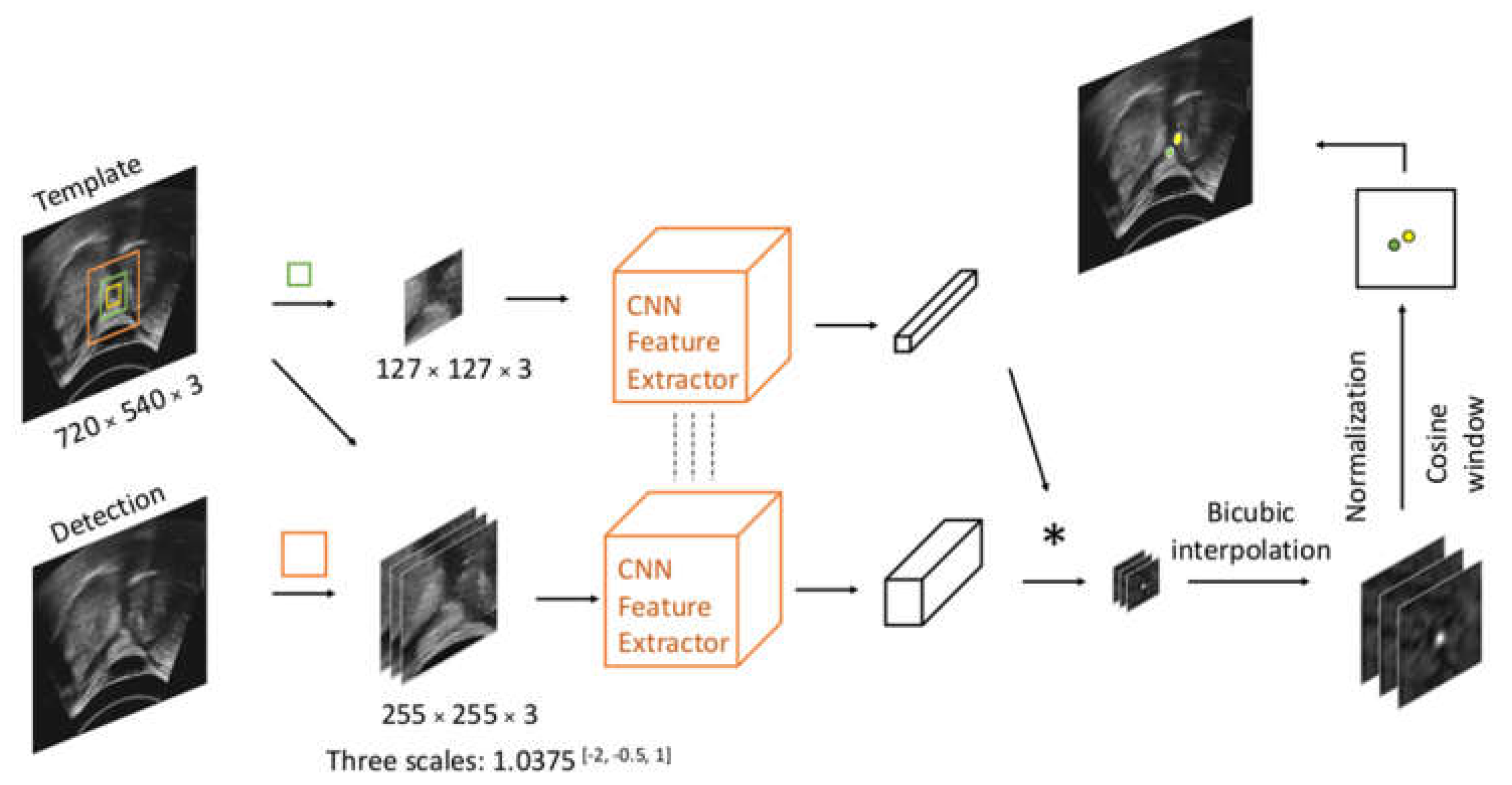
2.2.1. Siamese Trackers
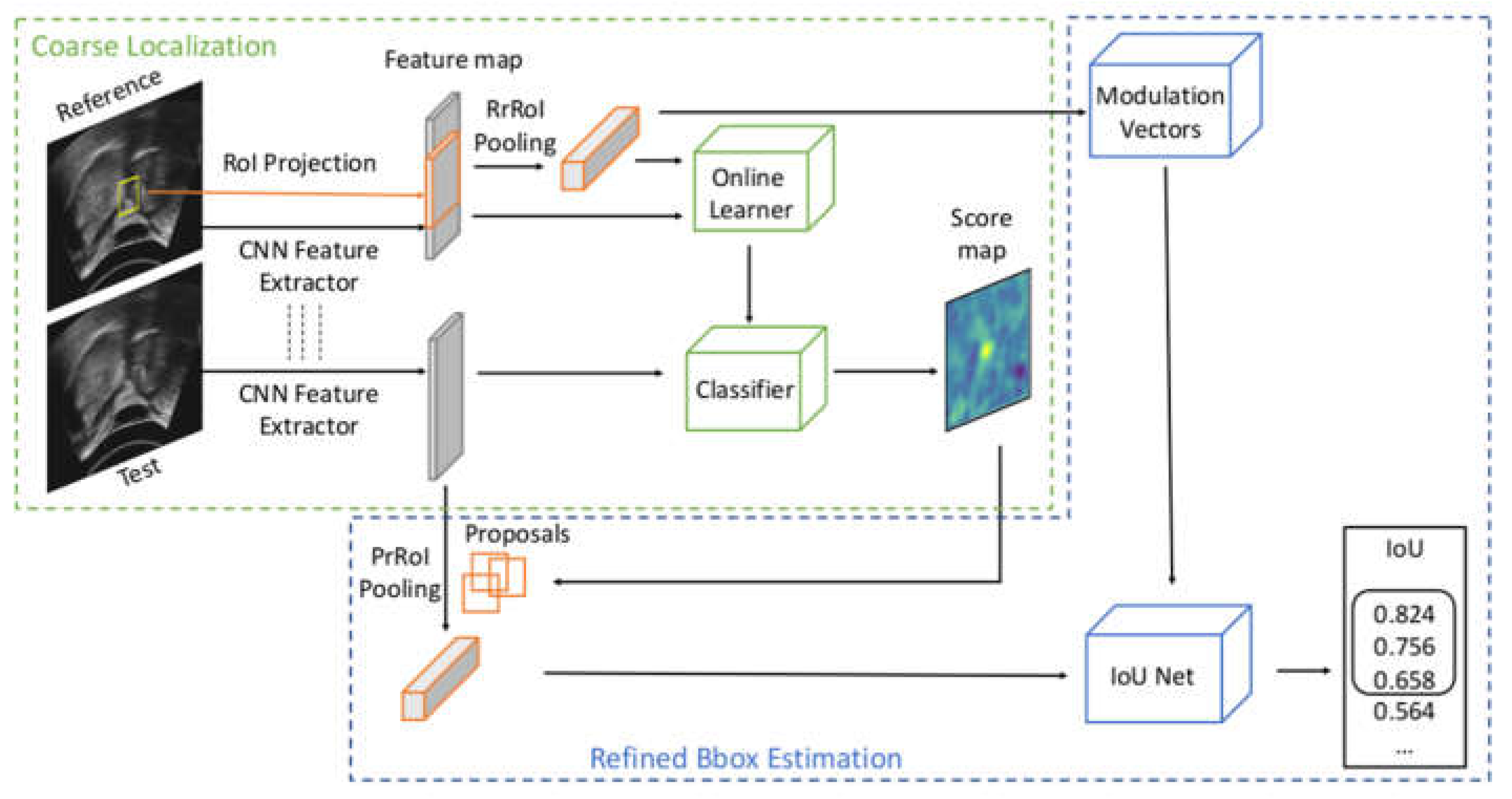
2.2.2. Multi-Stage Trackers
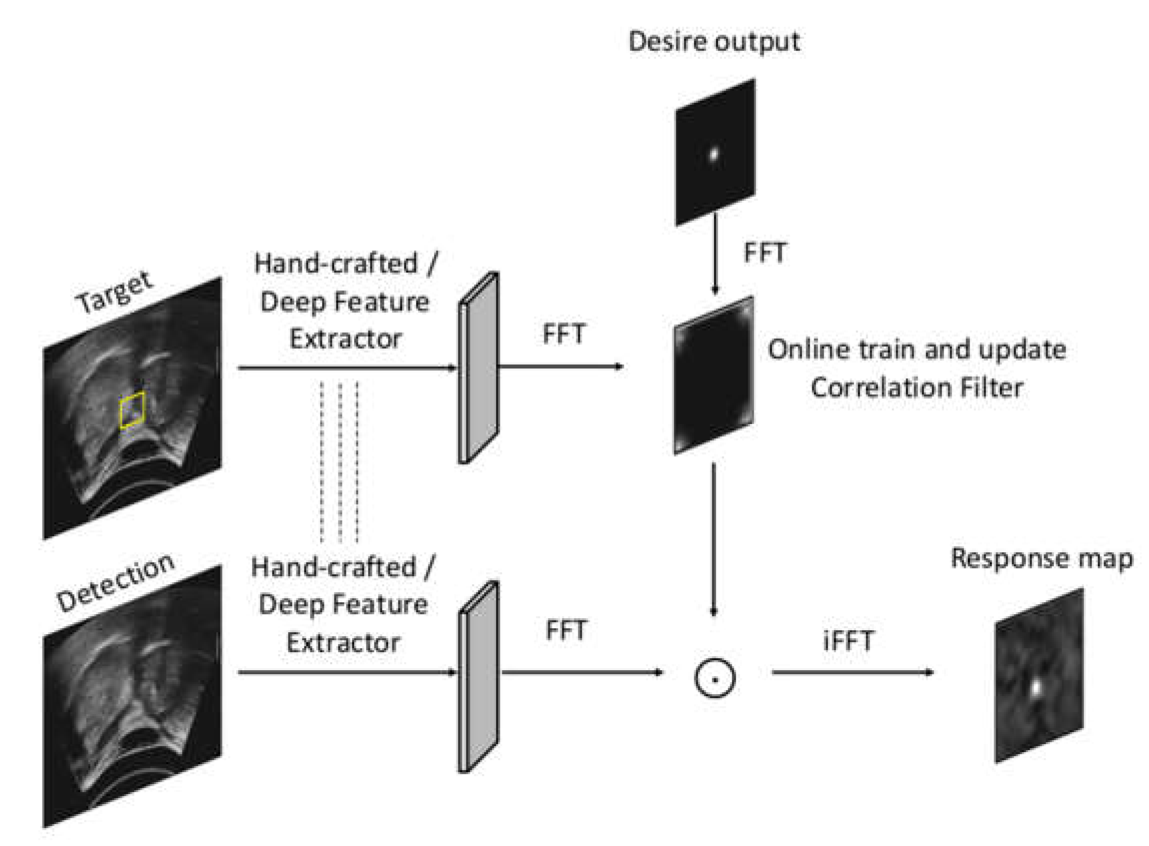
2.2.3. Correlation Filter Trackers
2.3. Implementation and Training Details of Deep Trackers
2.4. Evaluation
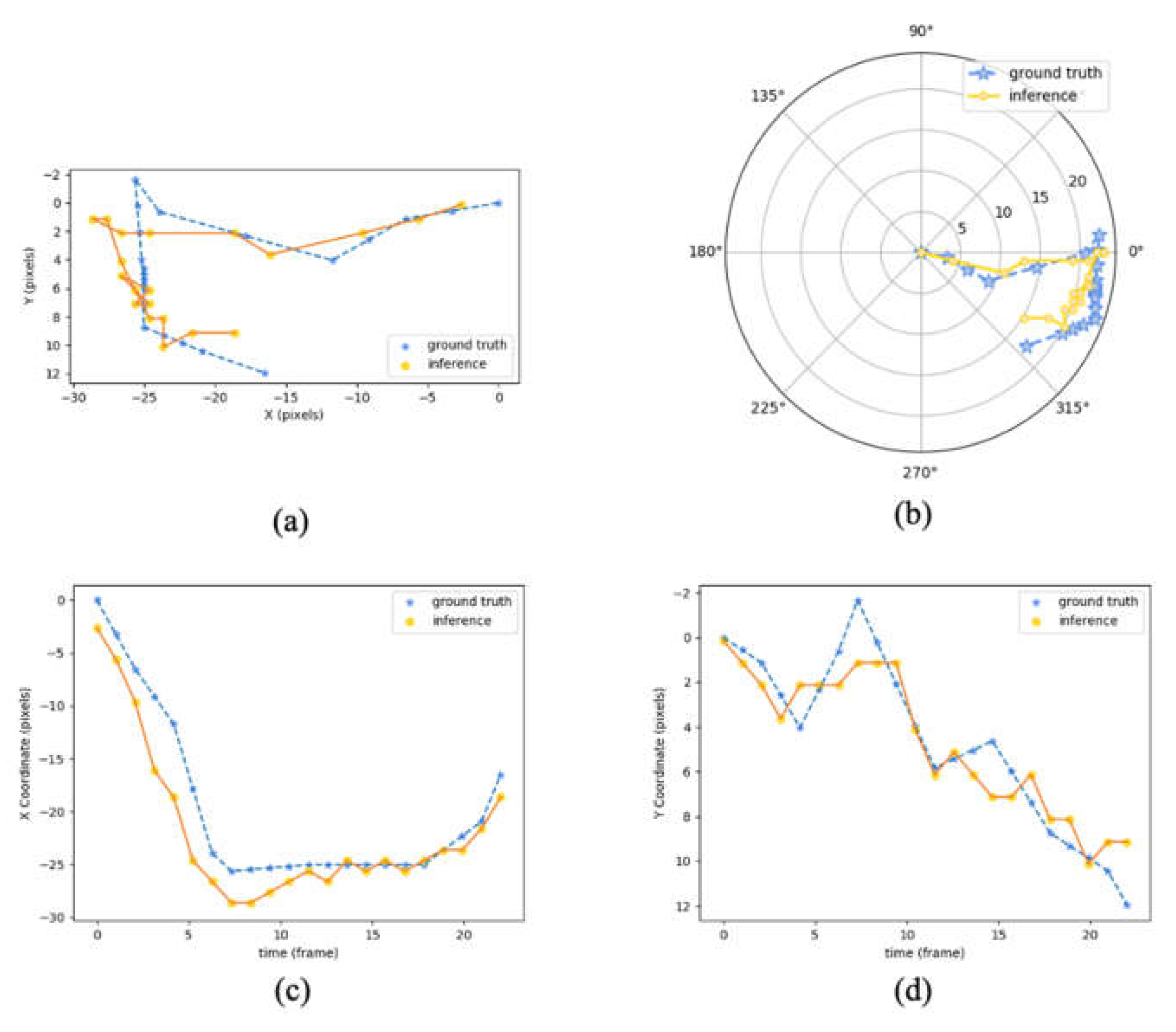
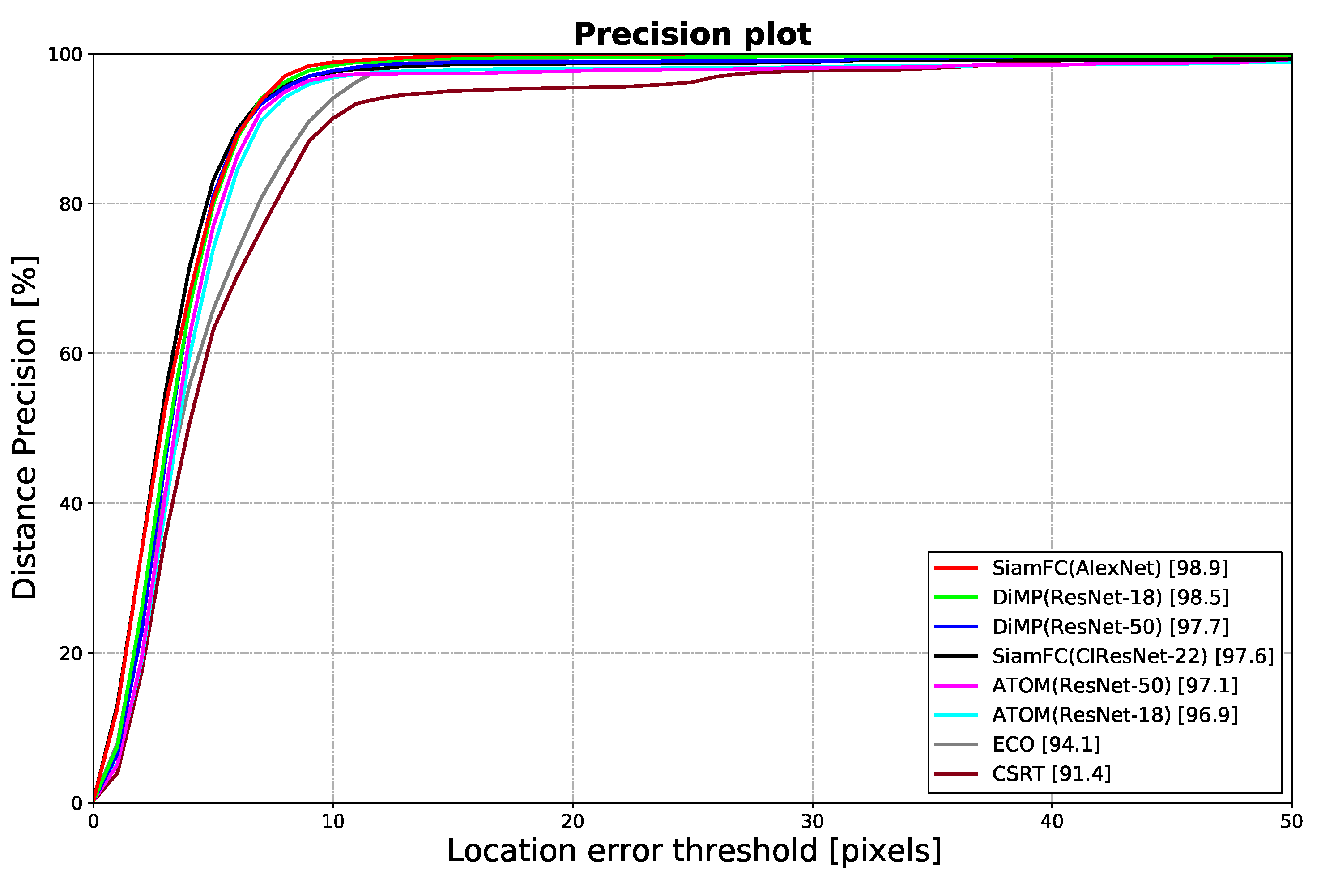
3. Results
4. Discussion
5. Conclusions
Supplementary Materials
Author Contributions
Funding
Institutional Review Board Statement
Informed Consent Statement
Data Availability Statement
Acknowledgments
Conflicts of Interest
References
- Smithard, D.G. Dysphagia: A Geriatric Giant? Med. Clin. Rev. 2016, 2, 1–7. [Google Scholar] [CrossRef]
- Bloem, B.R.; Lagaay, A.M.; Van Beek, W.; Haan, J.; Roos, R.A.; Wintzen, A.R. Prevalence of subjective dysphagia in community residents aged over 87. BMJ 1990, 300, 721. [Google Scholar] [CrossRef] [Green Version]
- Humbert, I.A.; Robbins, J. Dysphagia in the elderly. Phys. Med. Rehabil. Clin. N. Am. 2008, 19, 853–866. [Google Scholar] [CrossRef]
- O’Loughlin, G.; Shanley, C. Swallowing problems in the nursing home: A novel training response. Dysphagia 1998, 13, 172–183. [Google Scholar] [CrossRef]
- Martino, R.; Foley, N.; Bhogal, S.; Diamant, N.; Speechley, M.; Teasell, R. Dysphagia after stroke: Incidence, diagnosis, and pulmonary complications. Stroke 2005, 36, 2756–2763. [Google Scholar] [CrossRef] [Green Version]
- Sapir, S.; Ramig, L.; Fox, C. Speech and swallowing disorders in Parkinson disease. Curr. Opin. Otolaryngol. Head Neck Surg. 2008, 16, 205–210. [Google Scholar] [CrossRef] [PubMed]
- Azpeitia Armán, J.; Lorente-Ramos, R.M.; Gete García, P.; Collazo Lorduy, T.J.R. Videofluoroscopic evaluation of normal and impaired oropharyngeal swallowing. Radiographics 2019, 39, 78–79. [Google Scholar] [CrossRef] [PubMed]
- Marcotte, P. Critical Review: Effectiveness of FEES in Comparison to VFSS at Identifying Aspiration. 2007. Available online: https://www.uwo.ca/fhs/lwm/teaching/EBP/2006_07/Marcotte.pdf (accessed on 25 May 2021).
- Yoshida, M.; Miura, Y.; Yabunaka, K.; Sato, N.; Matsumoto, M.; Yamada, M.; Otaki, J.; Kagaya, H.; Kamakura, Y.; Saitoh, E.; et al. Efficacy of an education program for nurses that concerns the use of point-of-care ultrasound to monitor for aspiration and pharyngeal post-swallow residue: A prospective, descriptive study. Nurse Educ. Pract. 2020, 44, 102749. [Google Scholar] [CrossRef] [PubMed]
- Miura, Y.; Nakagami, G.; Tohara, H.; Ogawa, N.; Sanada, H. The association between jaw-opening strength, geniohyoid muscle thickness and echo intensity measured by ultrasound. Med. Ultrason. 2020, 22, 299–304. [Google Scholar] [CrossRef]
- Yabunaka, K.; Sanada, H.; Sanada, S.; Konishi, H.; Hashimoto, T.; Yatake, H.; Yamamoto, K.; Katsuda, T.; Ohue, M. Sonographic assessment of hyoid bone movement during swallowing: A study of normal adults with advancing age. Radiol. Phys. Technol. 2011, 4, 73–77. [Google Scholar] [CrossRef]
- Wintzen, A.R.; Badrising, U.A.; Roos, R.A.C.; Vielvoye, J.; Liauw, L. Influence of bolus volume on hyoid movements in normal individuals and patients with Parkinson’s disease. Can. J. Neurol. Sci. 1994, 21, 57–59. [Google Scholar] [CrossRef] [Green Version]
- Sonies, B.C.; Wang, C.; Sapper, D.J. Evaluation of normal and abnormal hyoid bone movement during swallowing by use of ultrasound duplex-Doppler imaging. Ultrasound Med. Biol. 1996, 22, 1169–1175. [Google Scholar] [CrossRef]
- Chi-Fishman, G.; Sonies, B.C. Effects of systematic bolus viscosity and volume changes on hyoid movement kinematics. Dysphagia 2002, 17, 278–287. [Google Scholar] [CrossRef] [PubMed]
- Yabunaka, K.; Konishi, H.; Nakagami, G.; Sanada, H.; Iizaka, S.; Sanada, S.; Ohue, M. Ultrasonographic evaluation of geniohyoid muscle movement during swallowing: A study on healthy adults of various ages. Radiol. Phys. Technol. 2012, 5, 34–39. [Google Scholar] [CrossRef] [PubMed]
- Perlman, A.L.; Booth, B.M.; Grayhack, J.P. Videofluoroscopic predictors of aspiration in patients with oropharyngeal dysphagia. Dysphagia 1994, 9, 90–95. [Google Scholar] [CrossRef]
- Hsiao, M.-Y.; Chang, Y.-C.; Chen, W.-S.; Chang, H.-Y.; Wang, T.-G. Application of ultrasonography in assessing oropharyngeal dysphagia in stroke patients. Ultrasound Med. Biol. 2012, 38, 1522–1528. [Google Scholar] [CrossRef]
- Lee, J.C.; Nam, K.W.; Jang, D.P.; Paik, N.J.; Ryu, J.S.; Kim, I.Y. A supporting platform for semi-automatic hyoid bone tracking and parameter extraction from videofluoroscopic images for the diagnosis of dysphagia patients. Dysphagia 2017, 32, 315–326. [Google Scholar] [CrossRef]
- Abdelrahman, A.S.; Abdeldayem, E.H.; Bassiouny, S.; Elshoura, H.M. Role of ultrasound in evaluation of pharyngeal dysphagia in children with cerebral palsy. Egypt. J. Radiol. Nucl. Med. 2019, 50, 1–6. [Google Scholar] [CrossRef] [Green Version]
- Hammond, R. A Pilot Study on the Validity and Reliability of Portable Ultrasound Assessment of Swallowing with Dysphagic Patients. Master’s Thesis, University of Canterbury, Christchurch, New Zealand, 2019. [Google Scholar]
- Lopes, M.I.; Silva, C.I.; Lima, L.; Lima, D.; Costa, B.; Magalhães, D.; Rodrigues, D.; Rêgo, T.I.; Pernambucano, L.; Santos, A. A deep learning approach to detect hyoid bone in ultrasound exam. In Proceedings of the 2019 8th Brazilian Conference on Intelligent Systems (BRACIS), Salvador, Brazil, 15–18 October 2019; pp. 551–555. [Google Scholar]
- Zhang, Z.; Coyle, J.L.; Sejdić, E. Automatic hyoid bone detection in fluoroscopic images using deep learning. Sci. Rep. 2018, 8, 12310. [Google Scholar] [CrossRef] [Green Version]
- Lee, D.; Lee, W.H.; Seo, H.G.; Oh, B.-M.; Lee, J.C.; Kim, H.C. Online learning for the hyoid bone tracking during swallowing with neck movement adjustment using semantic segmentation. IEEE Access 2020, 8, 157451–157461. [Google Scholar] [CrossRef]
- Bertinetto, L.; Valmadre, J.; Henriques, J.F.; Vedaldi, A.; Torr, P.H.S. Fully-convolutional siamese networks for object tracking. In Proceedings of the European Conference on Computer Vision, Amsterdam, The Netherlands, 8–16 October 2016; pp. 850–865. [Google Scholar]
- Danelljan, M.; Bhat, G.; Khan, F.S.; Felsberg, M. Atom: Accurate tracking by overlap maximization. In Proceedings of the IEEE/CVF Conference on Computer Vision and Pattern Recognition, Long Beach, CA, USA, 15–21 June 2019; pp. 4660–4669. [Google Scholar]
- Bhat, G.; Danelljan, M.; Gool, L.V.; Timofte, R. Learning discriminative model prediction for tracking. In Proceedings of the IEEE/CVF International Conference on Computer Vision, Seoul, Korea, 27 October–2 November 2019; pp. 6182–6191. [Google Scholar]
- Lukežič, A.; Vojíř, T.; Čehovin, L.; Matas, J.; Kristan, M. Discriminative correlation filter tracker with channel and spatial reliability. Int. J. Comput. Vis. 2018, 126, 671–688. [Google Scholar] [CrossRef] [Green Version]
- Danelljan, M.; Bhat, G.; Shahbaz Khan, F.; Felsberg, M. Eco: Efficient convolution operators for tracking. In Proceedings of the IEEE Conference on Computer Vision and Pattern Recognition, Honolulu, HI, USA, 21–26 July 2017; pp. 6638–6646. [Google Scholar]
- Bhat, G.; Johnander, J.; Danelljan, M.; Khan, F.S.; Felsberg, M. Unveiling the power of deep tracking. In Proceedings of the European Conference on Computer Vision (ECCV), Munich, Germany, 8–14 September 2018; pp. 483–498. [Google Scholar]
- Su, M.; Zheng, G.; Chen, Y.; Xie, H.; Han, W.; Yang, Q.; Sun, J.; Lv, Z.; Chen, J. Clinical applications of IDDSI framework for texture recommendation for dysphagia patients. J. Texture Stud. 2018, 49, 2–10. [Google Scholar] [CrossRef] [PubMed] [Green Version]
- Kwong, E.; Ng, K.-W.K.; Leung, M.-T.; Zheng, Y.-P. Application of ultrasound biofeedback to the learning of the mendelsohn maneuver in non-dysphagic adults: A pilot study. Dysphagia 2020. [Google Scholar] [CrossRef]
- Kristan, M.; Leonardis, A.; Matas, J.; Felsberg, M.; Pflugfelder, R.; Čehovin Zajc, L.; Vojir, T.; Hager, G.; Lukezic, A.; Eldesokey, A.; et al. The visual object tracking vot2017 challenge results. In Proceedings of the IEEE International Conference on Computer Vision Workshops, Venice, Italy, 22–29 October 2017; pp. 1949–1972. [Google Scholar]
- Hadfield, S.J.; Bowden, R.; Lebeda, K. The visual object tracking VOT2016 challenge results. Lect. Notes Comput. Sci. 2016, 9914, 777–823. [Google Scholar]
- Prashanth, H.S.; Shashidhara, H.L.; Murthy, K.N.B. Image scaling comparison using universal image quality index. In Proceedings of the 2009 International Conference on Advances in Computing, Control, and Telecommunication Technologies, Washington, DC, USA, 28–29 December 2009; pp. 859–863. [Google Scholar]
- Jiang, B.; Luo, R.; Mao, J.; Xiao, T.; Jiang, Y. Acquisition of localization confidence for accurate object detection. In Proceedings of the European Conference on Computer Vision (ECCV), Munich, Germany, 8–14 September 2018; pp. 784–799. [Google Scholar]
- Chen, Z.; Hong, Z.; Tao, D. An experimental survey on correlation filter-based tracking. arXiv 2015, arXiv:1509.05520. [Google Scholar]
- Chatfield, K.; Simonyan, K.; Vedaldi, A.; Zisserman, A. Return of the devil in the details: Delving deep into convolutional nets. arXiv preprint. arXiv 2014, arXiv:1405.3531. [Google Scholar]
- Danelljan, M.; Robinson, A.; Khan, F.S.; Felsberg, M. Beyond correlation filters: Learning continuous convolution operators for visual tracking. In Proceedings of the European Conference on Computer Vision, Amsterdam, The Netherlands, 8–16 October 2016; pp. 472–488. [Google Scholar]
- Krizhevsky, A.; Sutskever, I.; Hinton, G.E. Imagenet classification with deep convolutional neural networks. Adv. Neural Inf. Process. Syst. 2012, 25, 1097–1105. [Google Scholar] [CrossRef]
- Simonyan, K.; Zisserman, A. Very deep convolutional networks for large-scale image recognition. arXiv 2014, arXiv:1409.1556. [Google Scholar]
- He, K.; Zhang, X.; Ren, S.; Sun, J. Deep residual learning for image recognition. In Proceedings of the IEEE Conference on Computer Vision and Pattern Recognition, Las Vegas, NV, USA, 27–30 June 2016; pp. 770–778. [Google Scholar]
- Zhang, Z.; Peng, H. Deeper and wider siamese networks for real-time visual tracking. In Proceedings of the IEEE/CVF Conference on Computer Vision and Pattern Recognition, Long Beach, CA, USA, 15–20 June 2019; pp. 4591–4600. [Google Scholar]
- Huang, L. Siamfc-Pytorch. GitHub Repository. 2020. Available online: https://github.com/huanglianghua/siamfc-pytorch (accessed on 25 May 2021).
- Kingma, D.P.; Ba, J. Adam: A method for stochastic optimization. arXiv 2014, arXiv:1412.6980. [Google Scholar]
- Fan, H.; Lin, L.; Yang, F.; Chu, P.; Deng, G.; Yu, S.; Bai, H.; Xu, Y.; Liao, C.; Ling, H. Lasot: A high-quality benchmark for large-scale single object tracking. In Proceedings of the IEEE/CVF Conference on Computer Vision and Pattern Recognition, Long Beach, CA, USA, 15–20 June 2019; pp. 5374–5383. [Google Scholar]
- Wu, Y.; Lim, J.; Yang, M.-H. Online object tracking: A benchmark. In Proceedings of the IEEE Conference on Computer Vision and Pattern Recognition, Portland, OR, USA, 23–28 June 2013; pp. 2411–2418. [Google Scholar]
- Čehovin, L.; Leonardis, A.; Kristan, M. Visual object tracking performance measures revisited. IEEE Trans. Image Process. 2016, 25, 1261–1274. [Google Scholar]
- Wang, N.; Shi, J.; Yeung, D.-Y.; Jia, J. Understanding and diagnosing visual tracking systems. In Proceedings of the IEEE International Conference on Computer Vision, Las Condes, Chile, 7–13 December 2015; pp. 3101–3109. [Google Scholar]
- Kim, W.-S.; Zeng, P.; Shi, J.Q.; Lee, Y.; Paik, N.-J. Semi-automatic tracking, smoothing and segmentation of hyoid bone motion from videofluoroscopic swallowing study. PLoS ONE 2017, 12, e0188684. [Google Scholar] [CrossRef] [PubMed]
- Sia, I.; Carvajal, P.; Carnaby-Mann, G.D.; Crary, M.A. Measurement of hyoid and laryngeal displacement in video fluoroscopic swallowing studies: Variability, reliability, and measurement error. Dysphagia 2012, 27, 192–197. [Google Scholar] [CrossRef] [PubMed]
- Redmon, J.; Farhadi, A. Yolov3: An incremental improvement. arXiv 2018, arXiv:1506.01497. [Google Scholar]
- Ren, S.; He, K.; Girshick, R.; Sun, J. Faster r-cnn: Towards real-time object detection with region proposal networks. arXiv 2015, arXiv:1506.01497. [Google Scholar] [CrossRef] [PubMed] [Green Version]
- Liu, W.; Anguelov, D.; Erhan, D.; Szegedy, C.; Reed, S.; Fu, C.-Y.; Berg, A.C. Ssd: Single shot multibox detector. In Proceedings of the European Conference on Computer Vision, Amsterdam, The Netherlands, 8–16 October 2016; pp. 21–37. [Google Scholar]


| Tracking Methods | Precision at 10 Pixels ± SD (%) ↑ | Precision at 5 Pixels ± SD (%) ↑ | RMSE ± SD (Pixel) ↓ | AE ± SD (Pixel) ↓ | Pearson Correlation x-Axis ↑ | Pearson Correlation y-Axis ↑ | Relative Error of ROM in x-Axis (%) ↓ | Relative Error of ROM in y-Axis (%) ↓ | Relative Error of ROM (%) ↓ | Tracker Frame Rate (FPS) ↑ |
|---|---|---|---|---|---|---|---|---|---|---|
| SiamFC (AlexNet) | 98.9 ± 1.7 | 80.5 ± 18.9 | 3.85 ± 1.06 | 3.28 ± 1.10 | 0.985 ± 0.013 | 0.919 ± 0.034 | 13.3 ± 9.6 | 67.4 ± 70.1 | 9.5 ± 6.1 | 175 ± 2 |
| DiMP (ResNet-18) | 98.5 ± 3.3 | 79.9 ± 18.20 | 4.66 ± 2.24 | 3.65 ± 1.29 | 0.980 ± 0.013 | 0.883 ± 0.102 | 12.8 ± 8.2 | 69.8 ± 34.1 | 11.2 ± 7.7 | 63 ± 2 |
| DiMP (ResNet-50) | 97.7 ± 5.5 | 81.1 ± 15.6 | 4.95 ± 3.13 | 3.87 ± 1.61 | 0.979 ± 0.016 | 0.890 ± 0.123 | 14.4 ± 12.9 | 81.5 ± 85.4 | 14.4 ± 10.2 | 48 ± 1 |
| SiamFC (CIResNet-22) | 97.6 ± 3.2 | 83.2 ± 17.0 | 5.21 ± 3.59 | 3.64 ± 1.54 | 0.951 ± 0.109 | 0.735 ± 0.424 | 34.1 ± 83.1 | 157.5 ± 228.2 | 35.5 ± 90.8 | 116 ± 7 |
| ATOM (ResNet-50) | 97.1 ± 3.6 | 77.0 ± 18.8 | 7.93 ± 5.95 | 4.78 ± 1.81 | 0.910 ± 0.145 | 0.751 ± 0.243 | 28.8 ± 32.2 | 227.2 ± 391.3 | 21.2 ± 29.6 | 32 ± 2 |
| ATOM (ResNet-18) | 96.9 ± 3.4 | 74.0 ± 19.7 | 7.36 ± 4.35 | 4.71 ± 2.05 | 0.956 ± 0.061 | 0.734 ± 0.212 | 56.3 ± 84.7 | 229.6 ± 361.3 | 52.0 ± 89.8 | 43 ± 1 |
| ECO | 94.1 ± 12.8 | 65.8 ± 30.6 | 5.16 ± 2.16 | 4.43 ± 2.10 | 0.978 ± 0.021 | 0.890 ± 0.083 | 191 ± 18.7 | 150.4 ± 238.5 | 17.4 ± 13.6 | 24 ± 3 |
| CSRT | 91.4 ± 9.4 | 63.1 ± 25.3 | 8.23 ± 5.19 | 5.90 ± 2.75 | 0.922 ± 0.116 | 0.710 ± 0.263 | 27.6 ± 26.4 | 93.0 ± 100.9 | 26.9 ± 25.3 | 61 ± 3 |
Publisher’s Note: MDPI stays neutral with regard to jurisdictional claims in published maps and institutional affiliations. |
© 2021 by the authors. Licensee MDPI, Basel, Switzerland. This article is an open access article distributed under the terms and conditions of the Creative Commons Attribution (CC BY) license (https://creativecommons.org/licenses/by/4.0/).
Share and Cite
Feng, S.; Shea, Q.-T.-K.; Ng, K.-Y.; Tang, C.-N.; Kwong, E.; Zheng, Y. Automatic Hyoid Bone Tracking in Real-Time Ultrasound Swallowing Videos Using Deep Learning Based and Correlation Filter Based Trackers. Sensors 2021, 21, 3712. https://doi.org/10.3390/s21113712
Feng S, Shea Q-T-K, Ng K-Y, Tang C-N, Kwong E, Zheng Y. Automatic Hyoid Bone Tracking in Real-Time Ultrasound Swallowing Videos Using Deep Learning Based and Correlation Filter Based Trackers. Sensors. 2021; 21(11):3712. https://doi.org/10.3390/s21113712
Chicago/Turabian StyleFeng, Shurui, Queenie-Tsung-Kwan Shea, Kwok-Yan Ng, Cheuk-Ning Tang, Elaine Kwong, and Yongping Zheng. 2021. "Automatic Hyoid Bone Tracking in Real-Time Ultrasound Swallowing Videos Using Deep Learning Based and Correlation Filter Based Trackers" Sensors 21, no. 11: 3712. https://doi.org/10.3390/s21113712