Forecasting Coal Consumption in India by 2030: Using Linear Modified Linear (MGM-ARIMA) and Linear Modified Nonlinear (BP-ARIMA) Combined Models

Abstract

India’s coal consumption is closely related to greenhouse gas emissions and the balance of supply and demand in energy trading markets. Most existing research on India focuses on total energy, renewable energy and energy intensity. To fill this gap, this study used two single forecasting models: the metabolic grey model (MGM) and the Back-Pro-Pagation Network (BP) to make predictions. In addition, based on these two single models, this study also developed the ARIMA correction principle and derived two combined models: the metabolic grey model, the Autoregressive Integrated Moving Average model (MGM-ARIMA) and Back-Pro-Pagation Network; and the Autoregressive Integrated Moving Average model (BP-ARIMA). After fitting India’s coal consumption during 1995–2017, the average relative errors of the four models were 2.28%, 1.53%, 1.50% and 1.42% respectively. The forecast results show that coal consumption in India will continue to increase at an average annual rate of 2.5% during the period from 2018–2030.

1. Introduction

India, with a total population of more than 1.3 billion, has become the world’s third-largest emitter of greenhouse gases while rapidly industrializing and urbanizing. Coal is one of the most important causes of this problem. As the world’s second largest coal consumer and importer, India’s future coal changes will have a huge impact on the global coal trading market [1,2,3]. In addition, in terms of the impact on the domestic energy market, in 2016, India relied on coal to produce three-quarters of its electricity. This means that coal has an important supporting role in India, and that it impacts on the balance of supply and demand in the domestic energy market. Based on this situation, accurately predicting India’s future coal consumption is conducive to the formulation of both environmental and energy policy. On the one hand, controlling coal trends is beneficial to controlling India’s greenhouse gas emissions. On the other, determining changes in India’s relationship with coal plays an important role in controlling the global coal trading market ahead of time and balancing domestic energy supply and demand.

Most existing research focuses on the relationship between India’s energy intensity and economic development [4,5,6], renewable energy [7,8,9], and total energy consumption [2,10,11]. Few existing studies on Indian energy are focused on coal. For example, in terms of the relationship between energy and the economy, Ahmad et al. [12] studied the relationship between carbon emissions [13], energy consumption and economic development, and concluded that all energy sources have a positive impact on carbon emissions. Dasgupta et al. [14] derived and analyzed the energy intensity trends of seven energy-intensive manufacturing industries in India in the past. The conclusions show that structural changes have little effect on energy demand. In addition, there are also studies on the overall state of energy [15,16,17,18]. Wang et al. [19] predicted the total energy consumption of China and India. The research results show that India’s future energy growth rate will be 2–4 times that of China. Singh et al. [20] evaluated the potential index of solar energy development and provided reasonable suggestions for promoting solar energy development in India. Das et al. [21] constructed a modeling framework for linear dynamics and estimated India’s energy demand and carbon dioxide emissions for the cement industry in 2021. In terms of renewable energy [22,23,24], Sharma et al. [25] conducted a comprehensive assessment of the availability, environmental impact and development prospects of renewable energy in India. Sonal et al. [26] identified obstacles to solar energy development and provided countermeasures for India’s adoption of solar technology. Mohanty et al. [27] developed a new combination method based on statistical methods, fuzzy algorithms and neural networks, and applied it to solar forecasting in India. The results show that India’s future solar energy will rise to 35GW in 2020. Jiang et al. [28] developed and studied a multi-stage intelligent method based on integrated learning to predict 5-day global horizontal radiation in four regions of India. The final result confirms the effectiveness of the method. Bhattacharya and Ahmed [29] compared the return prediction performance of the GARCH model with the GARCH-ANN model using the root mean square error as a standard for crude oil prices in India. The results show that the hybrid model of ANN and EGARCH has the best performance.

In existing research on energy forecasting, most people use several single prediction methods. Few studies use multiple combined methods to predict the research object at the same time. For example, in the application of the grey model, Chen et al. [30] proposed two grey interval prediction methods: the interval grey model (abbreviated as: GM (1,1)) and the interval nonlinear grey Bernoulli model (NGBM (1,1)) for the problem of estimation range, which respectively predict minority and uncertain time series data. Yuan et al. [31] also used the GM (1,1) model and the Autoregressive Integrated Moving Average model (ARIMA) to predict the total energy consumption in China. The results show that China’s future energy consumption will grow at a rate of 4%. In the application of a neural network model, Jebaraj et al. [32] used a single neural network model to simultaneously predict and validate various energy sources in India. The verification results confirm that the neural network model can be make accurate predictions in most cases. Wang et al. [33] used the linear ARIMA to correct NMGM residuals to forecast China’s dependency on foreign oil; they reported that China’s dependency on foreign oil will exceed 80% of its energy expenditures by 2030. Hossain et al. [34] used artificial neural network models to simultaneously predict new solar and wind energy and applies them to the climate of Queensland. In the application of the ARIMA model, Oliveira et al. [35] used the bagging ARIMA model to predict medium- and long-term power consumption. Wang et al. [36] applied hybrid ARIMA and the metabolic grey technique to forecast shale gas output in the United States. Sen et al. [37] selected the correct ARIMA model and predicted energy consumption and greenhouse gas emissions of Indian pig iron manufacturing institutions. Li et al. [38] applied data mining and BP neural network models to the prediction of air pollution, and found the applicability of BP model to atmospheric data. Wang et al. [39] adopted single- and non-linear forecasting techniques to predict shale oil output in the United States. Xu et al. [40] adopted two single models: the ARIMA model and the BP neural network model to predict the monthly exchange rate of RMB. Through these applications, the study found that the average relative error of the two single models was 15% and 16%, respectively. Ray et al. [41] also used genetic algorithms and neural networks to predict electrical load, and found that genetic algorithms provide better prediction results than backpropagation.

Through combing the above literature, the following points can be summarized: (1) Existing forecasting literature on India is concentrated on renewable energy, carbon emissions and individual social issues. (2) The study of a single predictive model has been unable to meet the high-precision prediction effect. (3) The combined model has a good performance and is valued in the field of forecasting. Based on this, it can be observed that forecasting India’s coal consumption is a gap in current research, and the combined model can provide a tool for analyzing and predicting this research.

In order to fill this gap, this study intends to use a variety of mixed time series forecasting models to forecast India’s coal consumption in an all-round way. The innovations of this research are as follows. (1) This study used a high-precision mixed time series model to predict coal consumption in India. The forecast results will provide a reference for future energy planning and the economic development of India. (2) The model selected in this study includes two traditional single models: metabolic grey model (MGM) and Back-ProPagation Network (BP), and two newly-developed hybrid models based on the error correction principle: the metabolic grey model, Autoregressive Integrated Moving Average model (MGM-ARIMA) and Back-ProPagation Network, and the Autoregressive Integrated Moving Average model (BP-ARIMA). The simultaneous use of multiple models can provide exhaustive and comprehensive forecasting. It can also ensure the accuracy of forecasting and increase the credibility of the predicted data, which can provide an accurate reference for the development of follow-up policies.

The remainder of this paper is as follows: Section 2 categorizes the forecasting methods used. The introduction of the forecasting process is presented in Section 3. Section 4 introduces the accuracy and results of the predictions. A summary of the full text is given in Section 5.

2. Method

2.1. Metabolic Grey Model

The metabolic grey model (MGM) is an improvement to the traditional grey model (GM) by way of adding an element replacement process. The traditional grey model theory, abbreviated as the GM model, was developed in 1982 by Professor Deng Julong [42]. This theory mainly achieves an accurate understanding of system behavior through some known information. During operation, the GM model first accumulates or differentially processes a random sequence, making it regular: $x_k^1={\displaystyle \sum }_{i=1}^k{x}_i^0$. After that, a differential equation is established for this regular sequence: $\frac{d{x}^1}{dt}+a{x}^1=b$. Through the solution of the differential equation: ${\widehat{x}}_{k+1}^0=\left(1-e^a\right)\left({\widehat{x}}_1^0-\frac{b}{a}\right)e^{-ak}$, the prediction of the future data of the system can be realized. However, the GM model has obvious requirements for the predicted data. For example, the GM model is well suited to handle approximately 5–10 data. If the amount of data is too large or is fluctuating, the effect predicted by the GM model will be unsatisfactory.

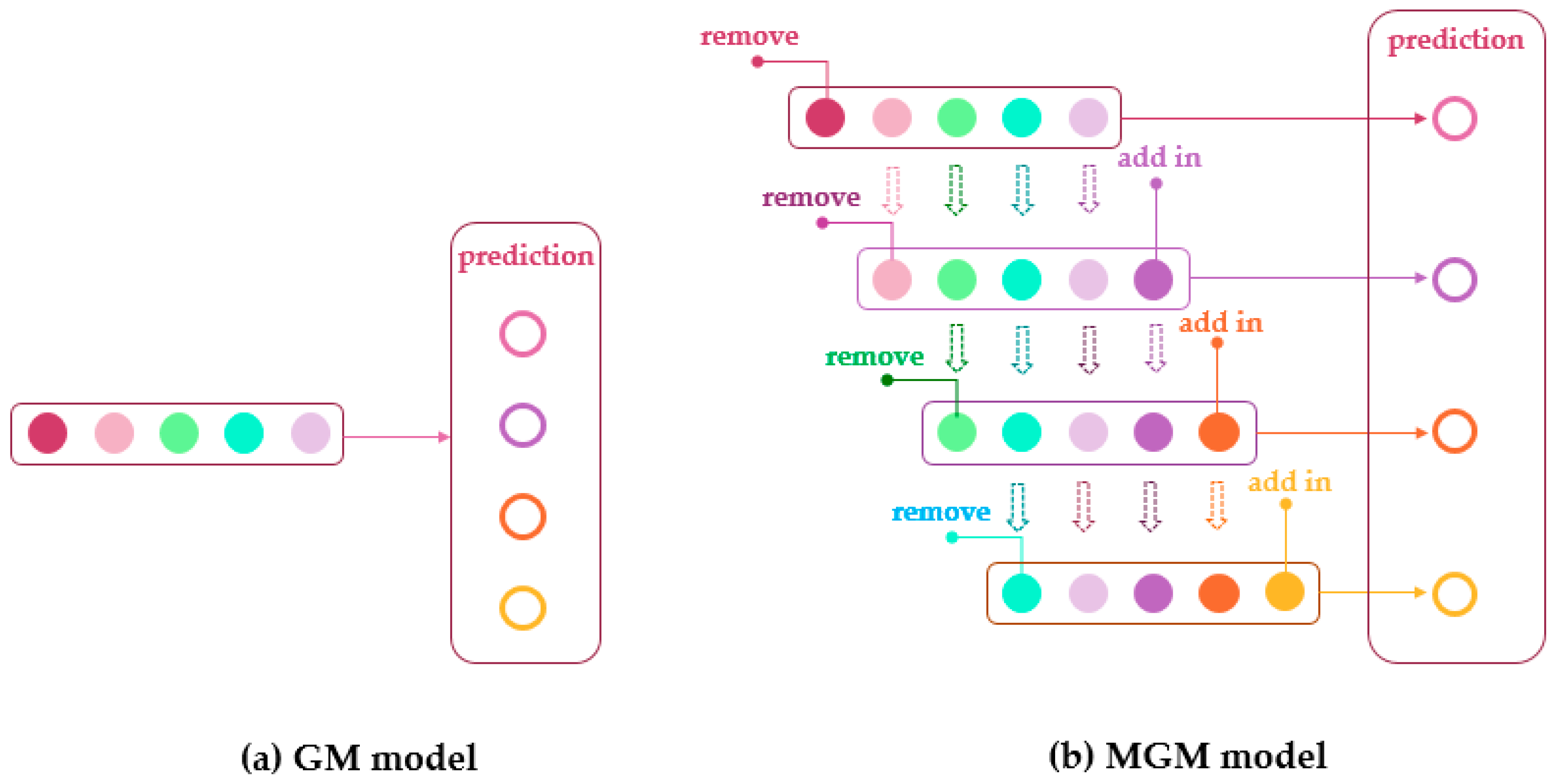
In order to solve this problem, data replacement can be added as a solution for the GM model. This improved model is called the metabolic grey model (abbreviated as the MGM model) [43]. The MGM model usually continues the calculation of the GM model in general. Specifically, the data processing method and the differential equation construction method of the MGM model are the same as the GM model. The difference is that the MGM model divides the prediction process of GM model into a number of prediction rounds, and the data used for each round of prediction is different. To illustrate the differences between the two models, Figure 1 shows the corresponding prediction processes of GM model and MGM model. Each colored circle represents a known block of data, while the open circle represents a block of data that needs to be predicted in the future.

As shown in Figure 1, the GM model uses only five pieces of data to predict all the unknown data. For MGM model, only one unknown piece of data is predicted per round. Furthermore, the data used by the GM model for prediction is invariant, and the data used for each round of the MGM model is different. The specific alternative principle is in line with the physiological process of metabolism. Assume the number of data used for grey prediction is five. After the first round of MGM model, the initial data is rejected, and the latest data reflecting the characteristics of the system is added. By analogy, each round of data sets used for MGM prediction is the one that best reflects system dynamics. This model overcomes a series of shortcomings of the traditional grey model for inaccurate prediction of large fluctuations in data. After this improvement, the MGM model can be applied to the prediction of large and volatile data sequences. The accuracy of the prediction is also greatly improved.

2.2. Back-ProPagation Network Forecasting Model

The Back-ProPagation Network, also known as the Back Propagation Neural Network, continuously corrects the network weights and thresholds by training the sample data to make the error function fall in the direction of the negative gradient and approach the desired output. It is a widely used neural network model, which is mostly used for function approximation, model recognition classification, data compression and time series prediction. The calculation process is as follows.

Step 1: Data preprocessing. In this step, the training data and test data are preprocessed using a normalized approach. After the model is established, the inverse normalization method can be used to restore the predicted data into meaningful data.

Step 2: Select the number of hidden layer neurons. Empirical formulas are often used as tools for this step: $\mathrm{n}=\sqrt{a+b}+c, n=\sqrt{ab}, n={\log }_{2}a$. Here, ‘a’ is assumed to be the number of neurons in the input layer, ‘n’ is the number of neurons in the hidden layer, and ‘b’ is the number of neurons in the output layer. After that, let ‘c’ take values from 1 to 10, constantly change ‘n’, and compare the models one by one to achieve the most accurate.

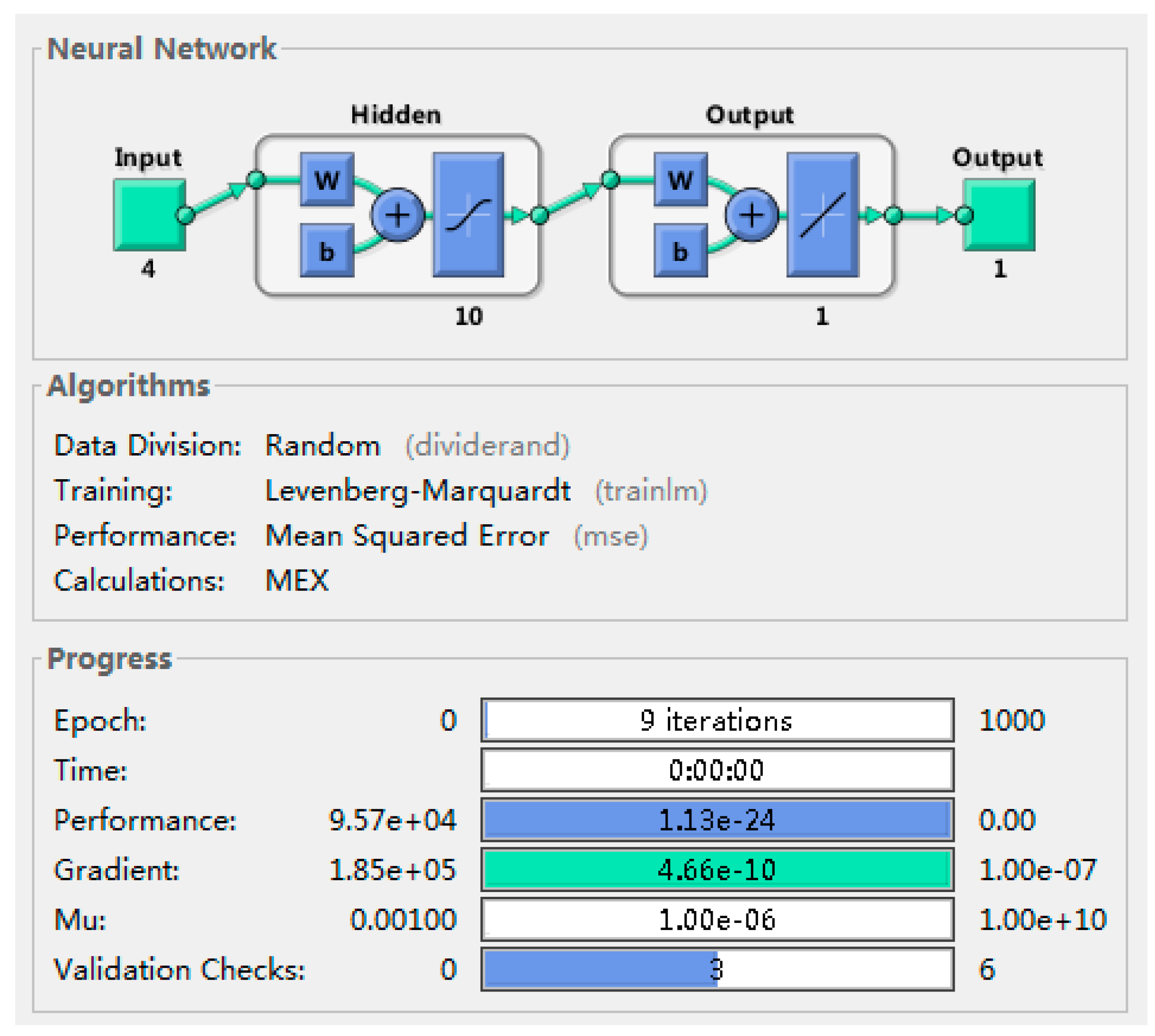
Step 3: Set parameters. In order to get the most effective model, it is often necessary to define the model during the training process. In this paper, the minimum training error is 1 × e⁻⁷, the number of training is 1000, and the learning rate is 0.01 (as shown in Figure 2).

Step 4: Model prediction and testing. In order to obtain a reasonably usable BP neural network model, it is necessary to judge the model by prediction and calculation error.

2.3. The Autoregressive Integrated Moving Average model

For time series predictions, the ARIMA model is one of the most commonly-used statistical models [44]. The principle of its prediction is to first convert a non-stationary time series into a stationary time series. Then, the dependent variable will be described as a model that only returns its lag value and the current and lag values of the random error term. It can be seen that the advantage of the ARIMA model is that the prediction process only requires endogenous variables and does not need other exogenous variables. However, the ARIMA model requires that the sequence be stable after being differentiated.

Specifically, the prediction process includes the following steps [39].

Step 1: Smooth the timing data with a differential tool. Stationarity serves to ensure that the fitted curve obtained by sampling time series can continue inertially along the existing form in a short time in the future, that is, the mean and variance of the data should not be excessively changed, theoretically.

Step 2: Establish an autoregressive model (AR). The autoregressive model is a model that describes the relationship between current value and historical value, and is a method of predicting itself by using the historical event data of the variable itself. Its formula is as follows:

$$y_t=\mu +{{\displaystyle \sum }}_{i=1}^p{\gamma }_i{y}_{t-i}+{ϵ}_t$$

(1)

where, $y_t$ is the current value; $\mu$ is constant term; p is the order; ${\gamma }_i$ is the autocorrelation coefficient; ${ϵ}_t$ is the errors.

Step 3: Establish a moving average model (MA). The moving average model focuses on the accumulation of error terms in the autoregressive model. It can effectively eliminate random fluctuations in predictions. Its formula is as follows:

$$y_t=\mu +{{\displaystyle \sum }}_{i=1}^q{\theta }_i{ϵ}_{t-i}+{ϵ}_t$$

(2)

Among them, the meaning of each letter is the same as (1), and ${\theta }_i$ is the correlation coefficient of the MA formula.

Step 4: Combine AR and MA, and construct an autoregressive moving average model (ARMA). The specific formula is as follows. In this formula, p and q are the orders of the autoregressive model and the moving average model, respectively. ${\gamma }_i$ and ${\theta }_i$ are the correlation coefficients of the two models, respectively, and need to be solved.

$$y_t=\mu +{{\displaystyle \sum }}_{i=1}^p{\gamma }_i{y}_{t-i}+{ϵ}_t+{{\displaystyle \sum }}_{i=1}^q{\theta }_i{ϵ}_{t-i}$$

(3)

2.4. Two Combined Linear Modified Linear (MGM-ARIMA) and Linear Modified Nonlinear (BP-ARIMA) Models

Although each single model has its own applicability, some inevitable flaws exist. In this case, the combined model comes out. A combined model can minimize the shortcomings of each single model and allow them to complement each other with the advantages of the two single models (as shown in

Table 1. Comparison of advantages and disadvantages between combined model and single model.

Type of Model		Advantage	Disadvantage
Single model	MGM	Easy to operate and dynamic	Unable to react to fluctuations
	ARIMA	Only need endogenous variables	Unable to react to nonlinear relationships
	BP	Self-learning and adaptability	Unpredictable prediction ability
Combined model	MGM-ARIMA	Only need endogenous variables, dynamic, can reflect nonlinear fluctuation data	Low fault tolerance
	BP-ARIMA	Good fault tolerance and can reflect nonlinear dynamic fluctuation data	General stability

) [45]. Generally speaking, common combinations of models: the equal weight method, minimum variance method, and so on. The predicted values produced by these methods are the results of combining individual prediction results after weighting based on precision.

Different from the traditional combinations, the approach used in this study is a combination of prediction steps [33]. Assume that the combined model includes two single models. The first model is called the base model, and the second is the modified model. The combined principle adopted in this study is to use the base model to make the prediction, and then use the modified model to recalibrate the error, i.e., in order to reduce the error. The specific steps are as follows.

Step 1: Use the base model to predict the original data sequence $X_t$. The prediction is done in the same way as the base model prediction step. At the end of this step, preliminary predictions $X_t^{*}$ are obtained.

Step 2: Calculate the predicted initial error. By comparing the prediction result with the real value, the prediction error of the base model can be obtained, and is called the initial error. The relevant formula is: $Y_t=X_t^{*}-X_t,\left(t=1,2,\cdots ,n\right).$ Where $Y_t$ is the error value corresponding to the response time point ‘t’, $X_t^{*}$ is the predicted value, and $X_t$ is the true value.

Step 3: The initial error sequence $Y_t$ is predicted by using modified model and a new error sequence $Y_t^{*}$ is obtained. Again, the modified model has the same processing steps as before. The error sequence obtained at this stage is called the new error sequence.

Step 4: Combine the preliminary predictions $X_t^{*}$ and the new error sequence $Y_t^{*}$, and obtain the final predictions based on this formula: $X_t^{**}=X_t^{*}+Y_t^{*},\left(t=1,2,\cdots ,n\right)$.

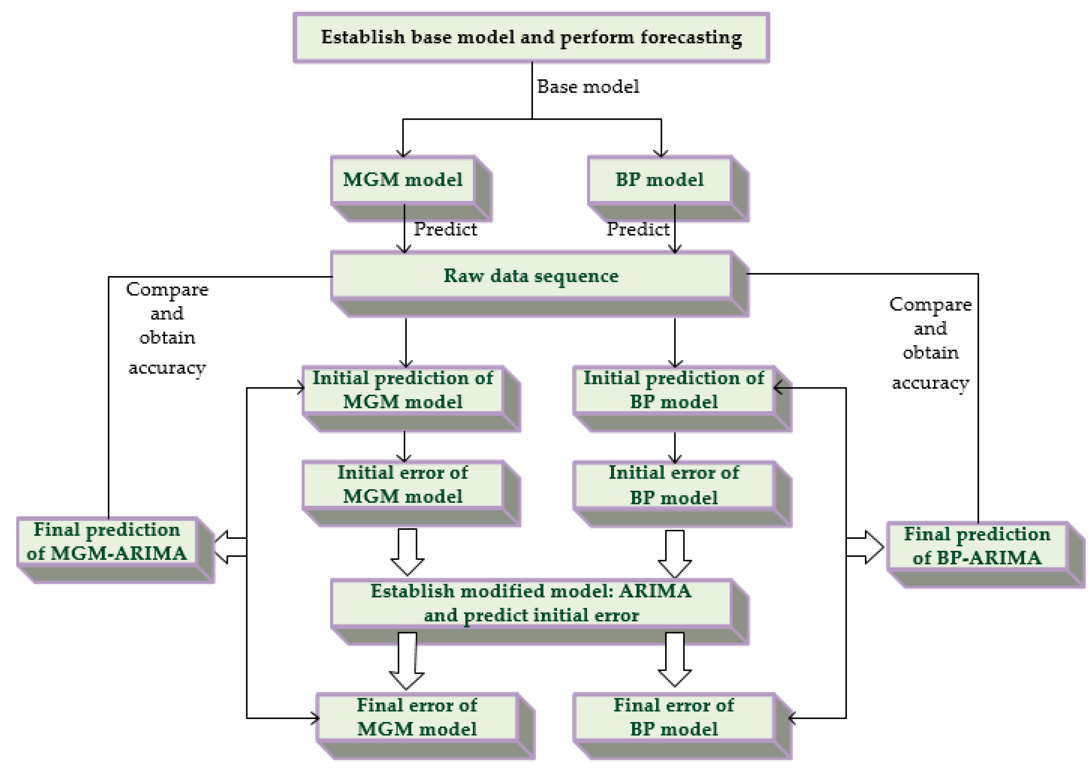
In this study, two combined linear modified linear (MGM-ARIMA) and linear modified nonlinear (BP-ARIMA) models were developed to predict India’s coal consumption. The similarity between the two models is that the modified models are all part of the ARIMA model. However, the difference is that the MGM-ARIMA model uses the MGM model as the base model, and the BP-ARIMA model uses the BP model as the base model. Since the principles of the three single models involved have already been explained before, Figure 3 will briefly introduce the main combination methods.

3. Forecasting Process and Empirical Results

The forecasting work of this study adopts the principle of “multi-model comparative prediction”. The forecasting tools used include two single models (MGM and BP model) and two combined models (MGM-ARIMA and BP-ARIMA). In conjunction with methods described in Section 2, a detailed forecast of coal consumption in India will be developed in this part.

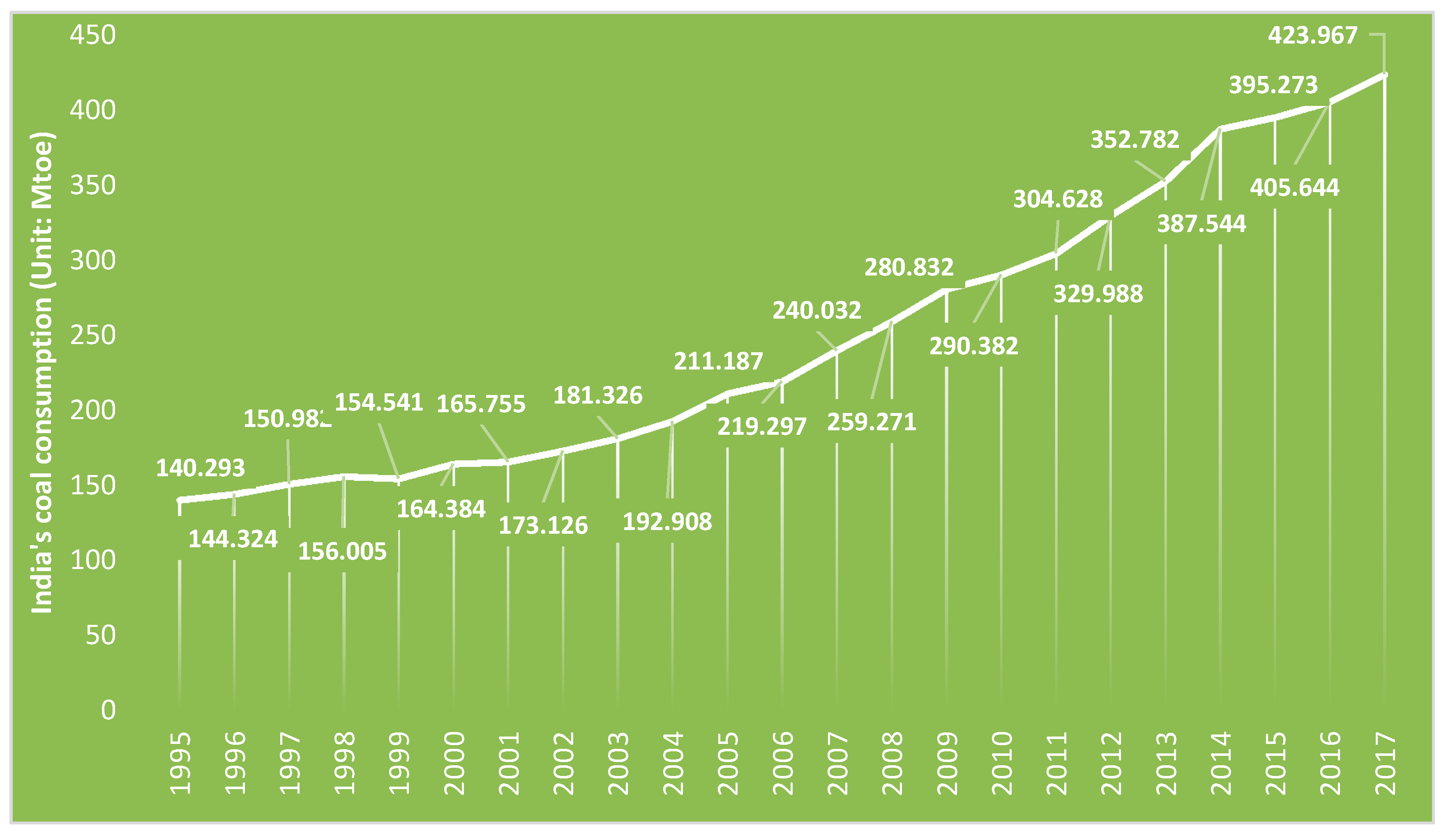
Figure 4 shows the trends in coal consumption in India in the period from 1995–2017. As seen in the figure, since 2000, India’s coal consumption has shown a steady upward trend. In the past three years, the growth rate has slowed down in 2014–2016, but a faster growth rate appeared again in 2017. This set of data is also used as raw data for multiple model predictions.

3.1. The Application of Metabolic Grey Model (MGM) in Forecasting India’s Coal Consumption

This study used five data blocks as the basis for each round of the MGM model prediction. According to the principle of metabolism, every five data used for calculation will produce a predicted result, and then five data blocks will be updated. Although the data blocks are constantly changing, each round of differential equation solving process is the same. The differential equation is as follows: $\frac{d{x}^{\left(1\right)}}{dt}+a{x}^{\left(1\right)}=b$. In order to get the predicted value, the unknown parameters ‘a’ and ‘b’ in this equation need to be solved. The number of groups obtained by the unknown parameter is the same as the number of rounds of data replacement.

Since the data interval used for prediction is 1995–2017, if based on five pieces of data, through software calculation, a total of 19 sets of parameters and 19 prediction results will be obtained (shown in

Table 2. The solution of parameters and predictions during MGM forecasting.

Forecasting Process	Solution of ‘a’	Solution of ‘b’	Forecasting Value	True Value	Relative Error
1995~1999→2000	−0.0233	141.2396	160.4866	164.384	2.371%
1996~2000→2001	−0.0249	145.2078	166.4489	165.755	0.419%
1997~2001→2002	−0.0245	148.7493	170.2216	173.126	1.678%
1998~2002→2003	−0.0346	147.9085	179.1436	181.326	1.203%
1999~2003→2004	−0.0343	154.3718	186.3309	192.908	3.410%
2000~2004→2005	−0.0505	152.534	201.8930	211.187	4.401%
2001~2005→2006	−0.067	154.1881	223.4998	219.297	1.917%
2002~2006→2007	−0.0654	164.6131	236.1804	240.032	1.604%
2003~2007→2008	−0.0694	174.6375	255.9016	259.271	1.299%
2004~2008→2009	−0.0716	186.8359	276.9859	280.832	1.369%
2005~2009→2010	−0.0815	193.9743	304.8337	290.382	4.977%
2006~2010→2011	−0.064	220.7369	313.1822	304.628	2.808%
2007~2011→2012	−0.051	243.497	321.7466	329.988	2.497%
2008~2012→2013	−0.0542	255.8387	344.4818	352.782	2.353%
2009~2013→2014	−0.0668	259.7517	376.2465	387.544	2.915%
2010~2014→2015	−0.0793	268.8488	417.1481	395.273	5.534%
2011~2015→2016	−0.0624	303.4909	427.1197	405.644	5.294%
2012~2016→2017	−0.0426	339.3002	428.0570	423.967	0.965%

).

According to the parameters of the second column and the third column in Table 2, the solution of the differential equation, that is, the predicted value, is obtained here. Comparing the predicted results of the metabolic grey model with the original true values, the relative error values indicate that the prediction effect of the MGM model is good.

3.2. The Application of Back-ProPagation Network Model (BP) in Forecasting India’s Coal Consumption

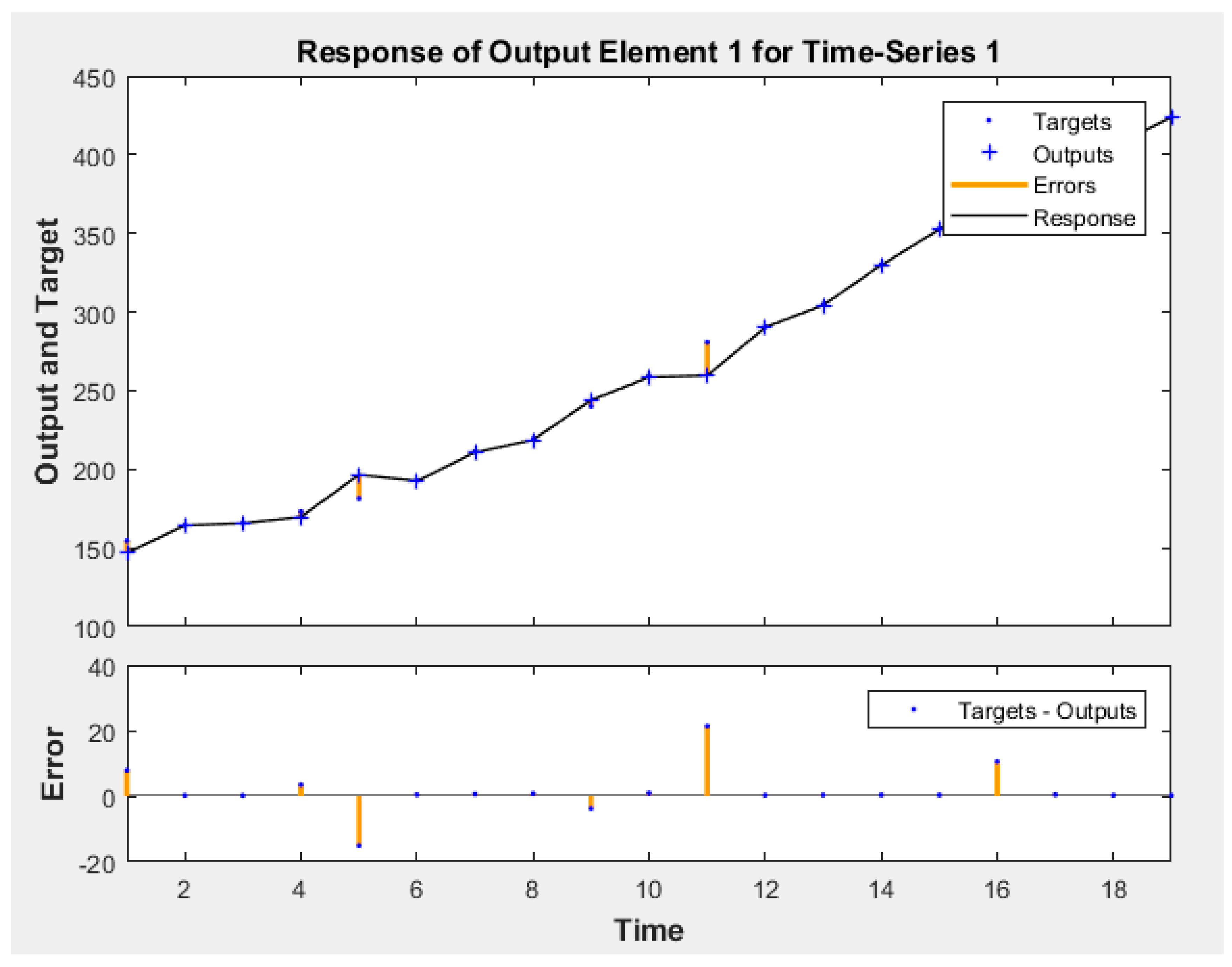
According to the method descripted above, the BP model needs to standardize the data before the operation. After that, a one-layer BP network was built [30]. The one-layer network includes an input layer, a hidden layer, and an output layer. For the number of neurons included in each layer of the network, the input layer contains 4 neurons, and both the hidden layer and the output layer contain 1 neuron. The settings of each aspect are as follows: the network hidden layer neuron transfer function uses ‘tansig’, the output layer neuron transfer function is ‘logsig’. The training function adopts ‘trainlm’, the minimum training error is 1 × e⁻⁷ and the number of training is 1000. After repeated training, the results of the final idealized model are shown in Figure 5. The error renderings in Figure 5 reflects the better model run results.

Due to the large volatility of the BP neural network itself, repeated training is required to achieve the desired result. After obtaining the desired results, inverse normalization is performed. The final predicted values are shown in

Table 3. Comparison of prediction results of BP model with real values.

Year	Forecasting Value	True Value	Relative Error
1999	154.5413	146.7572	5.037%
2000	164.3845	164.2484	0.083%
2001	165.7545	165.6686	0.052%
2002	173.1261	169.7080	1.974%
2003	181.3257	196.4610	8.347%
2004	192.9084	192.5092	0.207%
2005	211.1874	210.6085	0.274%
2006	219.2968	218.6137	0.311%
2007	240.0316	243.9196	1.620%
2008	259.2707	258.4555	0.314%
2009	280.8317	259.4844	7.601%
2010	290.3818	290.1657	0.074%
2011	304.6283	304.3510	0.091%
2012	329.9878	329.6839	0.092%
2013	352.7818	352.4987	0.080%
2014	387.5440	377.0672	2.703%
2015	395.2728	394.8589	0.105%
2016	405.6443	405.4386	0.051%
2017	423.8183	423.9675	0.035%

. The results in Table 3 show that, except for the relative error of individual years (such as 1999, 2003, 2009), the relative errors of the other years are less than 3%. This result proves that the prediction results obtained by the BP model are accurate.

3.3. The Application of Combined MGM-ARIMA Model in Forecasting India’s Coal Consumption

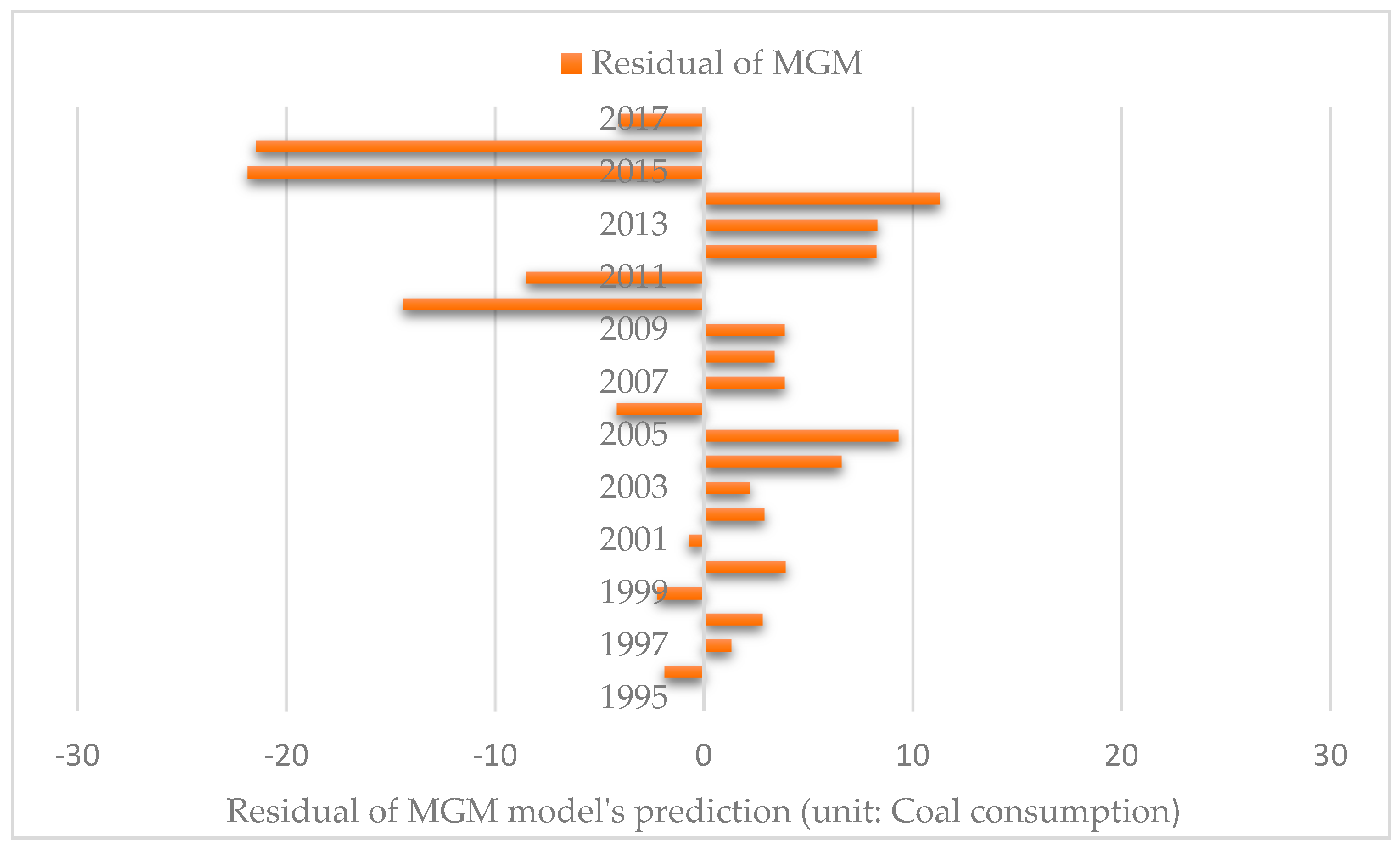
The combined MGM-ARIMA model uses the MGM model as the base model and uses the ARIMA model as the modified model. The forecasting process is a recalibration of the predicted results of the MGM model by the ARIMA model [36]. Combined with the predictions of the metabolic grey model in Section 3.1, the corresponding residual sequence is calculated and used to calculate modified ARIMA model.

Figure 6 shows the distribution of the residual sequence. The premise of processing with the ARIMA model is that the sequence is stationary. Obviously, the residual sequence in this figure is unstable, so a differential tool is needed to smooth the subsequence [46].

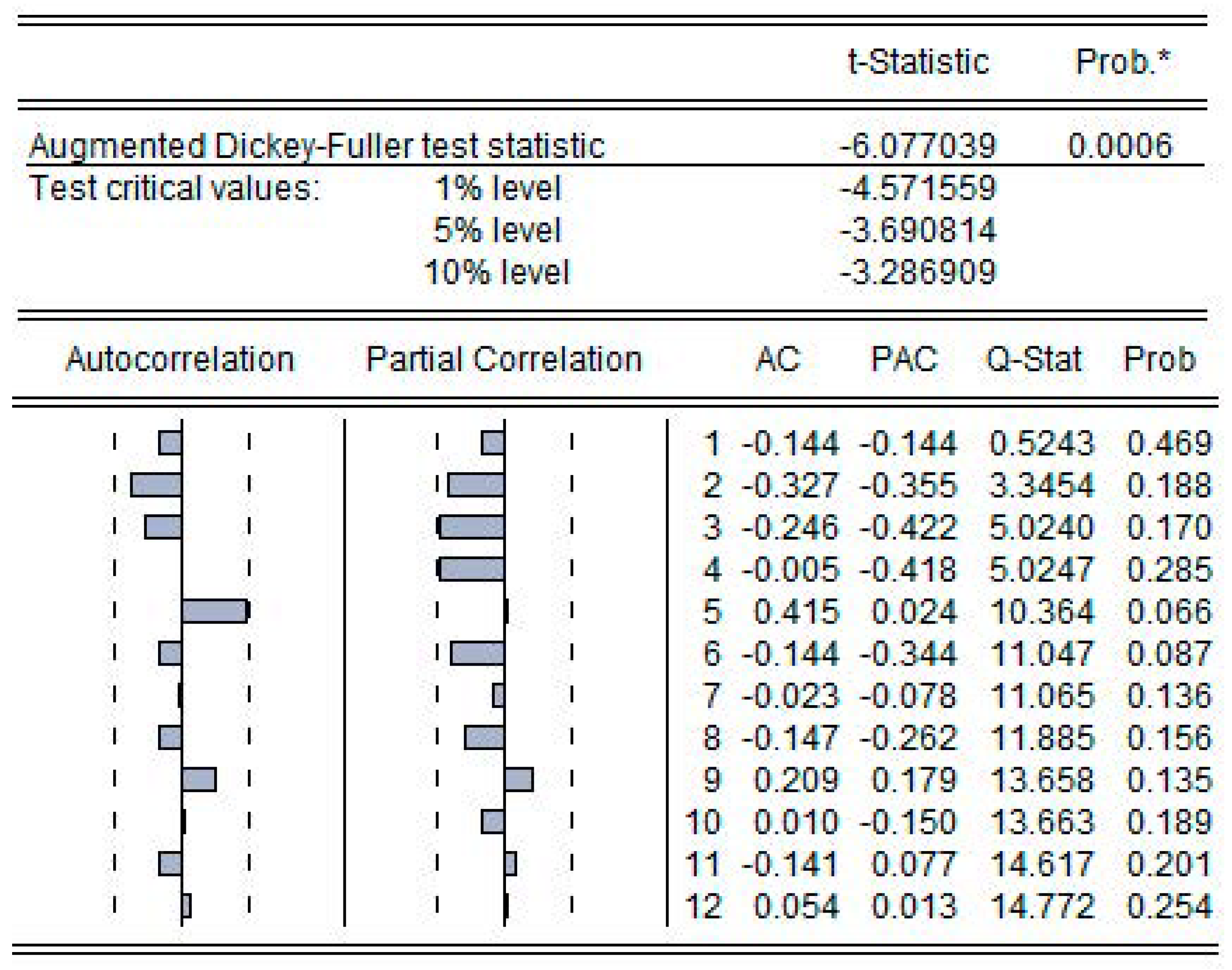
Figure 7 shows the results of first-order difference of this sequence. Two points of information can be drawn in this figure. First, the value of T-statistic is less than 1% test critical value, which is consistent with the inspection range. Second, the value of ‘P’ is 0.0006 < 0.01, which is also within the 1% confidence interval. The above two points prove that the sequence after the first order difference is stable, and that it satisfies the conditions of the next ARIMA model operation. That is, d = 1.

Next, the correlation coefficient map of the sequence after the difference is plotted. According to Figure 7, the case of the truncation determines the order of the autocorrelation coefficient and the partial autocorrelation coefficient. According to the relevant statistical principle, the autocorrelation coefficient graph represents the value of ‘q’, and the partial autocorrelation coefficient graph represents the value of ‘p’. The specific model types are determined as follows. When the autocorrelation coefficient graph is truncated and the autocorrelation graph is tailed, the model type is MA(q). When the autocorrelation coefficient graph is tailed and the autocorrelation graph is truncated, the model type is AR(p). When both are truncated, the model is ARMA(p,q). The autocorrelation coefficient map in Figure 7 suddenly shrinks to zero after the fifth order. At the same time, the partial autocorrelation coefficient graph suddenly shrinks to within two standard deviations after the fourth order. After repeated experiments, it was finally determined that the autocorrelation coefficient graph was truncated after the fifth order, and the partial autocorrelation coefficient graph was truncated after the fourth order. That is, p = 4, q = 5.

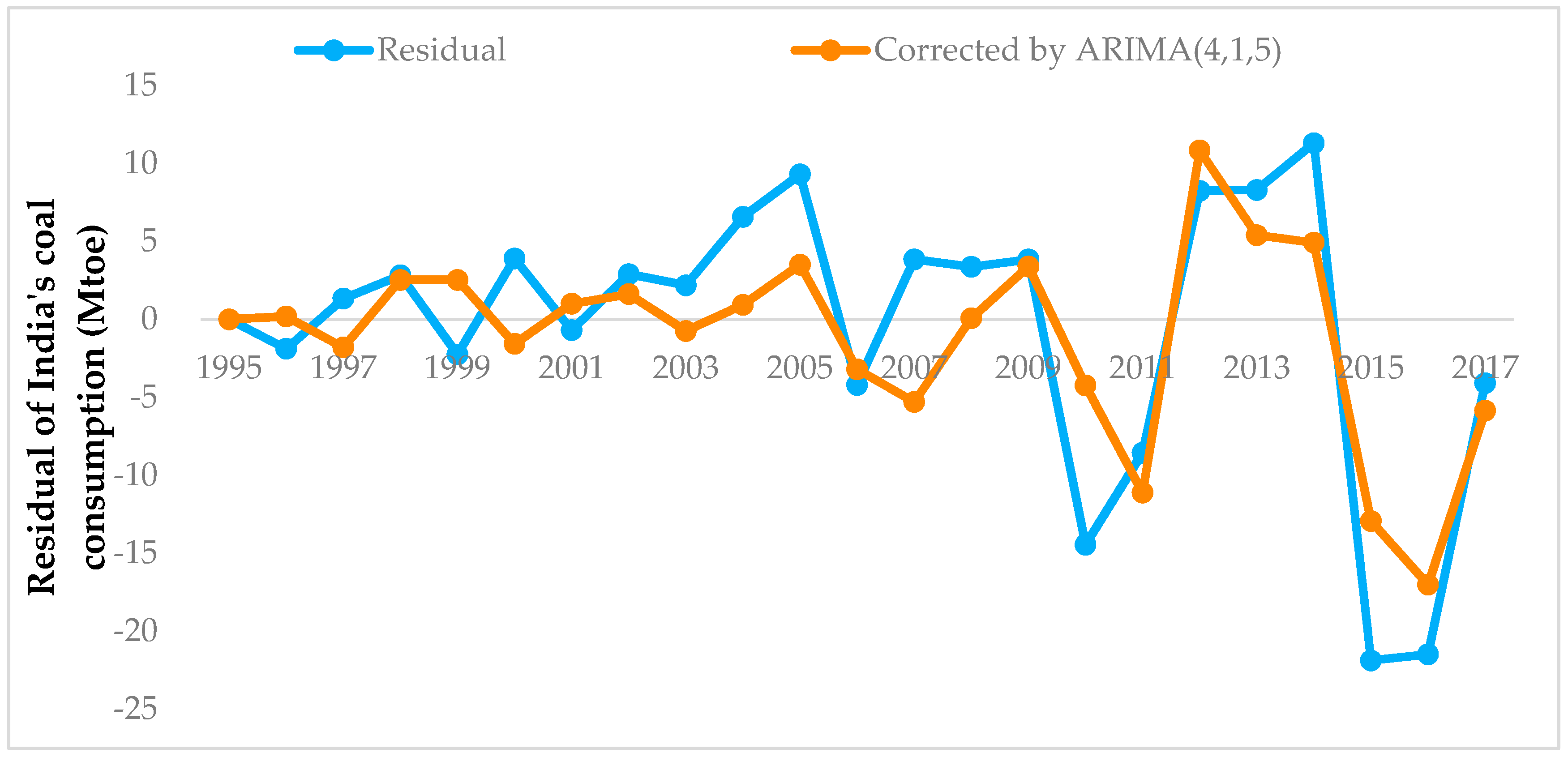
Since the order has been determined, ARIMA (4, 1, 5) is the final model for predicting the residual sequence. This model was run on the data in Figure 6 using SPSS software. After the operation, the corrected error results were obtained. Figure 8 compares the error curves before and after correction. Among them, the red curve is the corrected error, and the blue is the original error. As can be seen from the comparison chart, the red curve is usually more gradual than the blue curve. In other words, the correction effect of the ARIMA model does work.

After the preliminary prediction of the MGM model and the residual correction of the ARIMA model, the prediction results of the MGM-ARIMA model are shown in

Table 4. Comparison of prediction results of MGM-ARIMA model with real values.

Year	Forecasting Value	True Value	Relative Error
1995	140.2935	140.2935	0.000%
1996	144.1402	144.3235	0.127%
1997	152.7814	150.9822	1.192%
1998	153.4794	156.0052	1.619%
1999	152.0138	154.5413	1.635%
2000	165.9502	164.3845	0.952%
2001	164.7521	165.7545	0.605%
2002	171.5114	173.1261	0.933%
2003	182.0662	181.3257	0.408%
2004	191.9705	192.9084	0.486%
2005	207.6826	211.1874	1.660%
2006	222.4951	219.2968	1.458%
2007	245.3305	240.0316	2.208%
2008	259.2062	259.2707	0.025%
2009	277.4428	280.8317	1.207%
2010	294.6178	290.3818	1.459%
2011	315.7451	304.6283	3.649%
2012	319.1577	329.9878	3.282%
2013	347.3834	352.7818	1.530%
2014	382.6215	387.5440	1.270%
2015	408.2039	395.2728	3.271%
2016	422.6563	405.6443	4.194%
2017	429.8295	423.9675	1.383%

. In addition, Table 4 compares the ture values at the same time. By calculating the error formula, the relative error of the MGM-ARIMA model is maintained at about 1% on average.

3.4. The Application of Combined BP-ARIMA Model in Forecasting India’s Coal Consumption

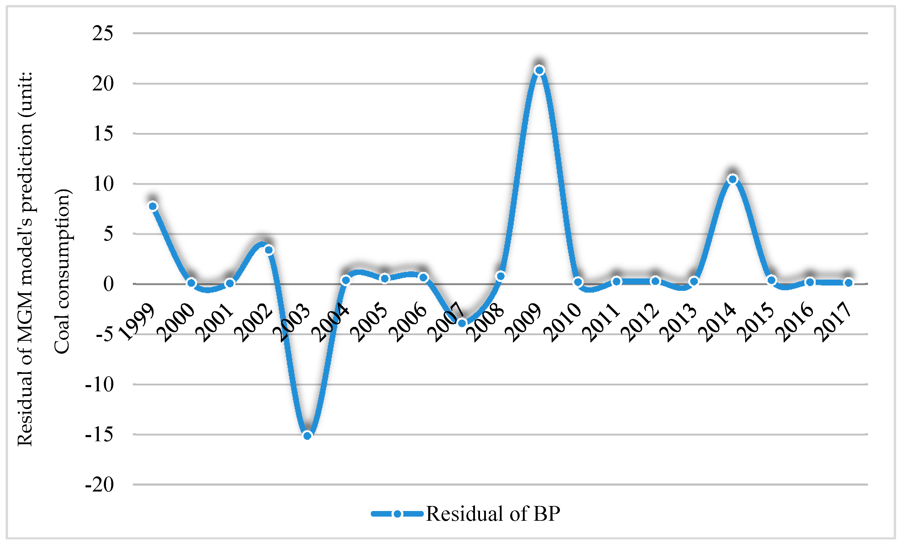
Based on Section 3.2, the combined BP-ARIMA uses ARIMA model to correct the predicted residuals of BP model. Subtracting the predicted values in Table 3 from the true values yields BP model’s residual sequence. Figure 9 depicts the trend of the residual sequence, and it is clear that this sequence is unstable.

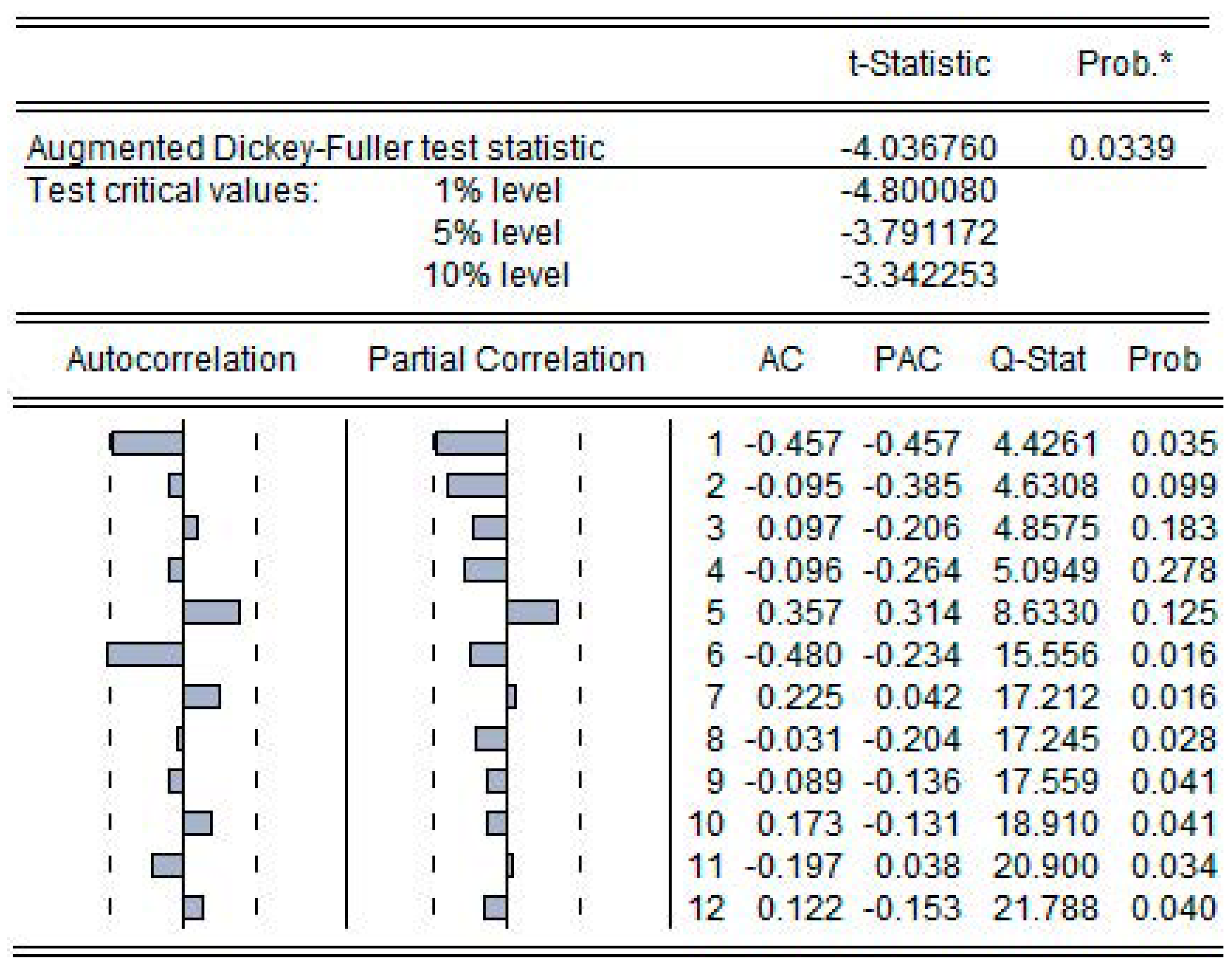
In order to smooth this residual sequence, it is necessary to implement the associated differential processing. Figure 10 shows the results of the first order difference of the residual sequence. As can be seen from the values in the figure, the t-statistic is less than 5% and greater than 1%. Therefore, a 95% confidence interval has been passed. This proves that the residual sequence is stationary after the first order difference and d = 1.

According to the judgment principle of ARIMA model parameters [38], a correlation diagram of the stationary sequence can be used to determine the values of ‘p’ and ‘q’. The autocorrelation coefficient graph in Figure 10 is suddenly censored around the sixth order. At the same time, the partial autocorrelation coefficient graph is truncated after the 1st order. After repeated verification, it is finally confirmed that the model with p = 1 and q = 6 has the highest accuracy.

Combine the BP prediction values in Table 3 with the ARIMA residual values run by the software. The predicted values of the BP-ARIMA model are shown in

Table 5. Comparison of prediction results of BP-ARIMA model with real values.

Year	Forecasting Value	True Value	Relative Error
1999	146.7572	154.5413	5.037%
2000	157.7795	164.3845	4.018%
2001	164.2612	165.7545	0.901%
2002	172.2478	173.1261	0.507%
2003	181.4857	181.3257	0.088%
2004	201.4915	192.9084	4.449%
2005	214.4971	211.1874	1.567%
2006	224.9321	219.2968	2.570%
2007	240.5080	240.0316	0.198%
2008	261.0766	259.2707	0.697%
2009	277.7586	280.8317	1.094%
2010	287.2930	290.3818	1.064%
2011	302.9228	304.6283	0.560%
2012	325.5480	329.9878	1.345%
2013	352.4511	352.7818	0.094%
2014	391.7261	387.5440	1.079%
2015	398.4748	395.2728	0.810%
2016	405.4416	405.6443	0.050%
2017	419.9612	423.9675	0.945%

. The relative error (a measure of prediction accuracy) is also listed in the table after comparison with actual values.

4. Analysis and Discussion

4.1. Comparison of Prediction Goodness of Four Models

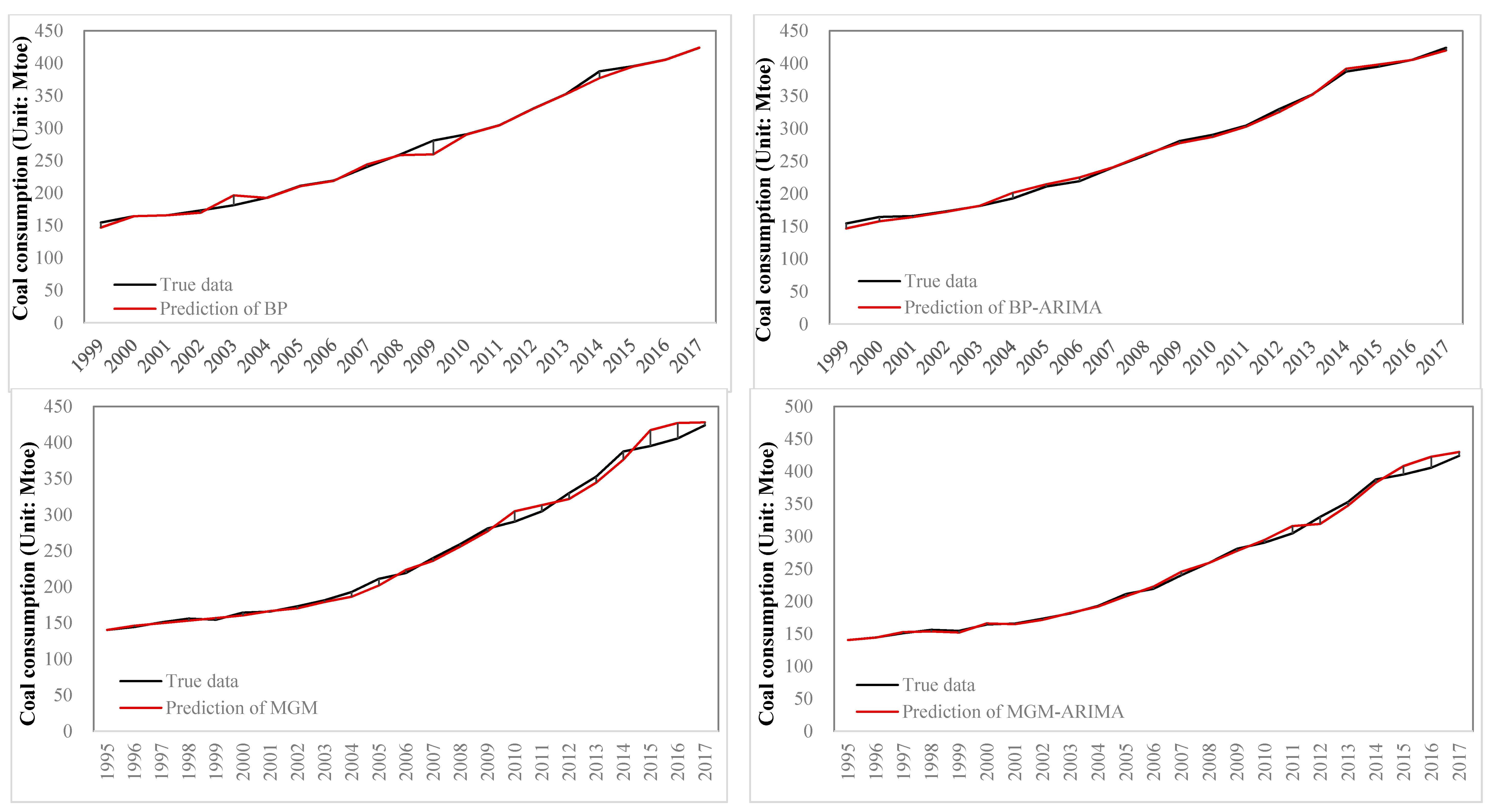
The forecasting process and results of each single model has been clearly shown in the previous section. However, by comparing the prediction results of the four models, the effects and differences between the model and the model can be reflected. Figure 11 illustrates the proximity of the predicted and actual values for each model using four sets of curves. This figure contains the following information. First, the predictions of the four models are all close to the real data. This usually reflects a good predictive effect. Second, by comparison with the naked eye, the combined model modified by the ARIMA model is closer to the true value than the uncorrected single model.

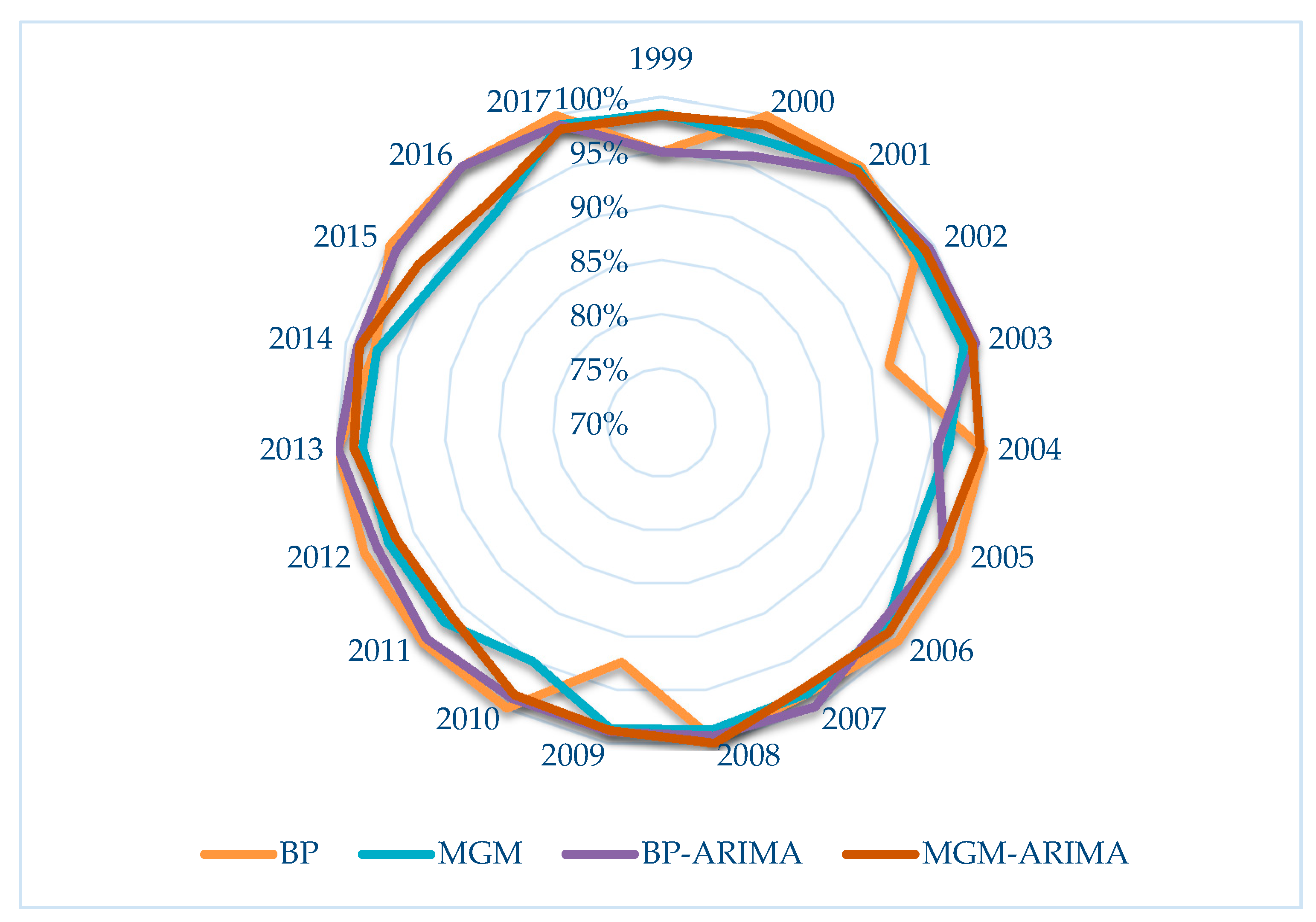
If measured by numerical values, the mean relative error can be used as the main indicator for judging the accuracy of prediction. Assume that the prediction accuracy is equal to 1 minus the relative error. Figure 12 compares the prediction accuracy of the four models per year. From the results shown in the figure, the minimum accuracy is higher than 90%. The accuracy is around 95%. The accuracy of this series shows that the predictions of the four models are all perfect.

A simultaneous comparison of prediction errors for single and combined models can reflect the relative prediction difference between the model and the model. If averaging the relative error of each year, the mean absolute percent error (MAPE) of each model can be calculated and used to reflect the predicted effect.

Table 6. The mean absolute percentage error of four models.

Type of Model	MAPE	Type of Model	MAPE
MGM	2.28%	BP	1.53%
MGM-ARIMA	1.50%√	BP-ARIMA	1.42%√

provides a comprehensive display of these values and reflects the following information. First, all MAPE values are within 5, which proves that the prediction data of all models is very reliable. Second, the average relative error of the combined model corrected by the ARIMA model is smaller than that of the uncorrected single model. In other words, the combined model does improve the single model. This means that the principle of error correction is feasible.

4.2. Forecasting Results of India’s Coal Consumption Period 2018–2030

The fitting phase is used to test the prediction error. The forecasting phase will be used to provide an outlook for future coal development.

Table 7. Future predictions obtained by the above four models.

Year	MGM	BP	MGM-ARIMA	BP-ARIMA
2018	433.968	426.264	449.667	428.918
2019	449.372	450.350	457.491	453.022
2020	464.568	451.690	443.763	437.731
2021	478.276	479.591	460.390	470.885
2022	494.675	479.698	480.468	462.969
2023	510.219	508.512	515.785	493.949
2024	526.441	509.129	523.187	497.852
2025	543.507	528.979	527.645	527.389
2026	560.707	539.927	541.423	534.732
2027	578.673	535.765	558.826	531.436
2028	597.185	559.112	592.722	554.876
2029	616.113	537.763	602.183	534.165
2030	635.731	542.302	620.357	539.110

summarizes the forecast data for the next 2018–2030. From the data shown in Table 7, although the results given by different models are different, the coal consumption in India still shows a clear upward trend in the future.

On the one hand, in terms of increments, in 2030, India’s coal consumption will increase by 150 million tons of oil equivalent compared to 2017. On the other, in terms of growth rate, India’s coal consumption will grow at an annual rate of 2.5% over the period of 2018–2030. This result is consistent with the future trend of Indian coal, as calculated by the International Energy Agency. According to the forecast of the International Energy Agency, coal consumption in India will grow at an annual rate of 3.9% in the future [47]. The growth rate predicted by this study is smaller than the value of the International Energy Agency. The reason for this difference is that India does not take into account the use of renewable energy in the future.

5. Conclusions

This study used a variety of models to fit the coal consumption of India during the period 1995–2017. After calculating the average relative error, the accuracy indicates that all four models are suitable for the prediction work done in this study. On this basis, the study used these four models to predict coal consumption in India from 2018–2030. Over all, this study has drawn the following conclusions in total.

(1)

After predicting two single models in the fitting stage, the average relative errors of the MGM and BP models were 2.28% and 1.53%, respectively, compared with the actual values.

(2)

Based on two single models of MGM and BP, the ARIMA correction principle was added to the development of the combined model. The MGM-ARIMA and BP-ARIMA models were developed and derived.

(3)

After the fitting stage is calculated, the average relative errors of the two combined models of MGM-ARIMA and BP-ARIMA are 1.50% and 1.42%, respectively. Comparing these two errors with 2.28% and 1.53%, this study found that the average relative error of each combined model is smaller than that of each single model. This proves that the combined model has an improved effect on a single model.

(4)

The study also applied the MGM, BP, MGM-ARIMA and BP-ARIMA models to predict coal consumption in India in the period from 2018–2030. The forecast results prove that India’s coal consumption will continue to grow at an average annual rate of 2.5%.

References

- IEA. Coal 2018; International Energy Agency: Paris, France, 2018. [Google Scholar]
- Wang, Q.; Li, R. Journey to burning half of global coal: Trajectory and drivers of China׳s coal use. Renew. Sustain. Energy Rev. 2016, 58, 341–346. [Google Scholar] [CrossRef]
- BP. BP Statistical Review of World Energy; British Petroleum: Londun, UK, 2018. [Google Scholar]
- Cheng, B.S. Causality between energy consumption and economic growth in India: An application of cointegration and error-correction modeling. Indian Econ. Rev. 1999, 34, 39–49. [Google Scholar]
- Wang, Q.; Su, M.; Li, R. Toward to economic growth without emission growth: The role of urbanization and industrialization in China and India. J. Clean. Prod. 2018, 205, 499–511. [Google Scholar] [CrossRef]
- Alam, M.J.; Begum, I.A.; Buysse, J.; Rahman, S.; Van Huylenbroeck, G. Dynamic modeling of causal relationship between energy consumption, CO2 emissions and economic growth in India. Renew. Sustain. Energy Rev. 2011, 15, 3243–3251. [Google Scholar] [CrossRef]
- Kumar, A.; Kumar, K.; Kaushik, N.; Sharma, S.; Mishra, S. Renewable energy in India: Current status and future potentials. Renew. Sustain. Energy Rev. 2010, 14, 2434–2442. [Google Scholar] [CrossRef]
- Pillai, I.R.; Banerjee, R. Renewable energy in India: Status and potential. Energy 2009, 34, 970–980. [Google Scholar] [CrossRef]
- Bhattacharya, S.; Jana, C. Renewable energy in India: Historical developments and prospects. Energy 2009, 34, 981–991. [Google Scholar] [CrossRef]
- Wu, L.; Liu, S.; Liu, D.; Fang, Z.; Xu, H. Modelling and forecasting CO2 emissions in the BRICS (Brazil, Russia, India, China, and South Africa) countries using a novel multi-variable grey model. Energy 2015, 79, 489–495. [Google Scholar] [CrossRef]
- Karmakar, S.; Suresh, M.V.J.J.; Kolar, A.K. The Effect of Advanced Steam Parameter-Based Coal-Fired Power Plants With Co2 Capture on the Indian Energy Scenario. Int. J. Green Energy 2013, 10, 1011–1025. [Google Scholar] [CrossRef]
- Ahmad, A.; Zhao, Y.; Shahbaz, M.; Bano, S.; Zhang, Z.; Wang, S.; Liu, Y. Carbon emissions, energy consumption and economic growth: An aggregate and disaggregate analysis of the Indian economy. Energy Policy 2016, 96, 131–143. [Google Scholar] [CrossRef]
- Wang, Q.; Chen, X. Energy policies for managing China’s carbon emission. Renew. Sustain. Energy Rev. 2015, 50, 470–479. [Google Scholar] [CrossRef]
- Dasgupta, S.; Roy, J. Analysing energy intensity trends and decoupling of growth from energy use in Indian manufacturing industries during 1973–1974 to 2011–2012. Energy Effic. 2016, 10, 925–943. [Google Scholar] [CrossRef]
- Peter, S.E.; Raglend, I.J. Sequential wavelet-ANN with embedded ANN-PSO hybrid electricity price forecasting model for Indian energy exchange. Neural Comput. Appl. 2017, 28, 1–16. [Google Scholar] [CrossRef]
- Luthra, S.; Mangla, S.K.; Kharb, R.K. Sustainable assessment in energy planning and management in Indian perspective. Renew. Sustain. Energy Rev. 2015, 47, 58–73. [Google Scholar] [CrossRef]
- Jena, S.; Kumar, A.; Singh, J.K.; Mani, I. Biomechanical model for energy consumption in manual load carrying on Indian farms. Int. J. Ind. Ergon. 2016, 55, 69–76. [Google Scholar] [CrossRef]
- Raj, A.S.; Oliver, D.H.; Srinivas, Y. Forecasting groundwater vulnerability in the coastal region of southern Tamil Nadu, India—a fuzzy-based approach. Arabian J. Geosci. 2016, 9, 351. [Google Scholar] [CrossRef]
- Wang, Q.; Li, S.; Li, R. Forecasting energy demand in China and India: Using single-linear, hybrid-linear, and non-linear time series forecast techniques. Energy 2018, 161, 821–831. [Google Scholar] [CrossRef]
- Singh, A.; Vats, G.; Khanduja, D. Exploring tapping potential of solar energy: Prioritization of Indian states. Renew. Sustain. Energy Rev. 2016, 58, 397–406. [Google Scholar] [CrossRef]
- Das, A.; Kandpal, T.C. A model to estimate energy demand and CO2 emissions for the Indian cement industry. Int. J. Energy Res. 2015, 23, 563–569. [Google Scholar] [CrossRef]
- Luthra, S.; Kumar, S.; Garg, D.; Haleem, A. Barriers to renewable/sustainable energy technologies adoption: Indian perspective. Renew. Sustain. Energy Rev. 2015, 41, 762–776. [Google Scholar] [CrossRef]
- Hammar, L.; Ehnberg, J.; Mavume, A.; Cuamba, B.C.; Molander, S. Renewable ocean energy in the Western Indian Ocean. Renew. Sustain. Energy Rev. 2012, 16, 4938–4950. [Google Scholar] [CrossRef]
- Kumar, V.S.; Anoop, T.R. Wave energy resource assessment for the Indian shelf seas. Renew. Energy 2015, 76, 212–219. [Google Scholar] [CrossRef]
- Sharma, N.K.; Tiwari, P.K.; Sood, Y.R. Promotion of renewable energy in Indian power sector moving towards deregulation. Appl. Mech. Rev. 2012, 61, 129–137. [Google Scholar]
- Sindhu, S.; Nehra, V.; Luthra, S. Identification and analysis of barriers in implementation of solar energy in Indian rural sector using integrated ISM and fuzzy MICMAC approach. Renew. Sustain. Energy Rev. 2016, 62, 70–88. [Google Scholar] [CrossRef]
- Mohanty, S.; Patra, P.K.; Sahoo, S.S.; Mohanty, A. Forecasting of solar energy with application for a growing economy like India: Survey and implication. Renew. Sustain. Energy Rev. 2017, 78, 539–553. [Google Scholar] [CrossRef]
- Jiang, H.; Dong, Y.; Xiao, L. A multi-stage intelligent approach based on an ensemble of two-way interaction model for forecasting the global horizontal radiation of India. Energy Convers. Manag. 2017, 137, 142–154. [Google Scholar] [CrossRef]
- Bhattacharya, S.; Ahmed, A. Forecasting crude oil price volatility in India using a hybrid ANN-GARCH model. Int. J. Bus. Forecast. Mark. Intell. 2018, 4, 446–457. [Google Scholar] [CrossRef]
- Yong, B.; Xu, Z.; Shen, J.; Chen, H.; Tian, Y.; Zhou, Q. Neural network model with Monte Carlo algorithm for electricity demand forecasting in Queensland. In Proceedings of the Australasian Computer Science Week Multiconference, Geelong, Australia, 30 January–3 February 2017; p. 47. [Google Scholar]
- Yuan, C.; Liu, S.; Fang, Z. Comparison of China’s primary energy consumption forecasting by using ARIMA (the autoregressive integrated moving average) model and GM(1,1) model. Energy 2016, 100, 384–390. [Google Scholar] [CrossRef]
- Jebaraj, S.; Iniyan, S.; Kota, H. Forecasting of commercial energy consumption in India using Artificial Neural Network. Int. J. Glob. Energy Issues 2007, 27, 276–301. [Google Scholar] [CrossRef]
- Wang, Q.; Li, S.; Li, R. China’s dependency on foreign oil will exceed 80% by 2030: Developing a novel NMGM-ARIMA to forecast China’s foreign oil dependence from two dimensions. Energy 2018, 163, 151–167. [Google Scholar] [CrossRef]
- Hossain, R.; Ooa, A.M.T.; Alia, A.B.M.S. Historical Weather Data Supported Hybrid Renewable Energy Forecasting using Artificial Neural Network (ANN). Energy Procedia 2012, 14, 1035–1040. [Google Scholar] [CrossRef] [Green Version]
- Oliveira, E.M.D.; Oliveira, F.L.C. Forecasting mid-long term electric energy consumption through bagging ARIMA and exponential smoothing methods. Energy 2018, 144, 776–788. [Google Scholar] [CrossRef]
- Wang, Q.; Li, S.; Li, R.; Ma, M. Forecasting U.S. shale gas monthly production using a hybrid ARIMA and metabolic nonlinear grey model. Energy 2018, 160, 378–387. [Google Scholar] [CrossRef]
- Sen, P.; Roy, M.; Pal, P. Application of ARIMA for forecasting energy consumption and GHG emission: A case study of an Indian pig iron manufacturing organization. Energy 2016, 116, 1031–1038. [Google Scholar] [CrossRef]
- Li, A.; Xu, X. A New PM2.5 Air Pollution Forecasting Model Based on Data Mining and BP Neural Network Model. In Proceedings of the 2018 3rd International Conference on Communications, Information Management and Network Security (CIMNS 2018); Available online: https://doi.org/10.2991/cimns-18.2018.25 (accessed on 28 January 2019).
- Wang, Q.; Song, X.; Li, R. A novel hybridization of nonlinear grey model and linear ARIMA residual correction for forecasting U.S. shale oil production. Energy 2018, 165, 1320–1331. [Google Scholar] [CrossRef]
- Xu, M.; Li, W. Research on Exchange Rate Forecasting Model Based on ARIMA Model and Artificial Neural Network Model. In Proceedings of the 2017 2nd International Conference on Materials Science, Machinery and Energy Engineering (MSMEE 2017); Available online: https://doi.org/10.2991/msmee-17.2017.225 (accessed on 28 January 2019).
- Ray, P.; Mishra, D.P.; Lenka, R.K. Short term load forecasting by artificial neural network. In Proceedings of the 2016 International Conference on Next Generation Intelligent Systems (ICNGIS), Kottayam, India, 1–3 September 2016; pp. 1–6. [Google Scholar]
- Deng, J. Grey System Fundamental Method; Huazhong University of Science and Technology: Wuhan, China, 1982. [Google Scholar]
- Zhai, J.; Sheng, J. Gray Model and Application of MGM (1, n). Syst. Eng. Theory Pract. 1997, 17, 109–113. [Google Scholar]
- Box, G.E.P.; Jenkins, G. Time Series Analysis, Forecasting and Control; Holden-Day, Inc.: San Francisco, CA, USA, 1990; pp. 238–242. [Google Scholar]
- Wang, Q.; Li, S.; Li, R. Will Trump’s coal revival plan work?—Comparison of results based on the optimal combined forecasting technique and an extended IPAT forecasting technique. Energy 2019, 169, 762–775. [Google Scholar] [CrossRef]
- Zuo, X. Research on Theory and Application of Unit Root Test; Huazhong University of Science and Technology: Wuhan, China, 2012. [Google Scholar]
- IEA. Global Coal Demand is Forecast to be Stable through 2023. Available online: https://www.iea.org/coal2018/ (accessed on 24 January 2019).
Figure 1.
Improvement of MGM Model based on GM Model. (Note: Each circle represents a single piece of data.)
Figure 2.
The parameters set by the BP model.
Figure 3.
The combination mode and operation flow of the MGM-ARIMA and BP-ARIMA model.
Figure 4.
Raw data on coal consumption in India (Unit: Mtoe). (Source: BP Statistical Review of World Energy 2018 [3]).
Figure 5.
Prediction effect of BP model derived from Matlab software.
Figure 6.
The prediction error derived from the MGM model.
Figure 7.
First-order difference results and correlation coefficient graph of MGM residual sequence.
Figure 8.
A comparison of the MGM residuals before and after ARIMA correction.
Figure 9.
The prediction error derived from the BP model.
Figure 10.
First-order difference results and correlation coefficient graph of BP residual sequence.
Figure 11.
Comparison of four model fitting effects.
Figure 12.
Comparison of predicted accuracy of four models in each year.